- Forums
- Product Forums
- General Purpose MicrocontrollersGeneral Purpose Microcontrollers
- i.MX Forumsi.MX Forums
- QorIQ Processing PlatformsQorIQ Processing Platforms
- Identification and SecurityIdentification and Security
- Power ManagementPower Management
- Wireless ConnectivityWireless Connectivity
- RFID / NFCRFID / NFC
- Advanced AnalogAdvanced Analog
- MCX Microcontrollers
- S32G
- S32K
- S32V
- MPC5xxx
- Other NXP Products
- S12 / MagniV Microcontrollers
- Powertrain and Electrification Analog Drivers
- Sensors
- Digital Signal Controllers
- Vybrid Processors
- ColdFire/68K Microcontrollers and Processors
- 8-bit Microcontrollers
- PowerQUICC Processors
- OSBDM and TBDML
- S32M
-
- Solution Forums
- Topics
- Mobile Robotics - Drones and RoversMobile Robotics - Drones and Rovers
- NXP Training ContentNXP Training Content
- University ProgramsUniversity Programs
- Rapid IoT
- NXP Designs
- SafeAssure-Community
- OSS Security & Maintenance
- Using Our Community
-
- Software Forums
- MCUXpresso Software and ToolsMCUXpresso Software and Tools
- CodeWarriorCodeWarrior
- MQX Software SolutionsMQX Software Solutions
- Model-Based Design Toolbox (MBDT)Model-Based Design Toolbox (MBDT)
- FreeMASTER
- eIQ Machine Learning Software
- Embedded Software and Tools Clinic
- S32 SDK
- S32 Design Studio
- GUI Guider
- Zephyr Project
- Voice Technology
- Application Software Packs
- Secure Provisioning SDK (SPSDK)
- Processor Expert Software
-
- Cloud Lab Forums
-
- Knowledge Bases
- ARM Microcontrollers
- Identification and Security
- i.MX Processors
- Model-Based Design Toolbox (MBDT)
- QorIQ Processing Platforms
- S32 Automotive Processing Platform
- CodeWarrior
- Wireless Connectivity
- MCUXpresso Suite of Software and Tools
- MQX Software Solutions
- RFID / NFC
- Advanced Analog
-
- Home
- :
- Model-Based Design Toolbox (MBDT)
- :
- Model-Based Design Toolbox (MBDT)
- :
- Re: Module 9: Position Observer (Part 2/2)
Module 9: Position Observer (Part 2/2)
- Subscribe to RSS Feed
- Mark Topic as New
- Mark Topic as Read
- Float this Topic for Current User
- Bookmark
- Subscribe
- Mute
- Printer Friendly Page
Module 9: Position Observer (Part 2/2)
- Mark as New
- Bookmark
- Subscribe
- Mute
- Subscribe to RSS Feed
- Permalink
- Report Inappropriate Content
The first part of this article can be found here: Module 9: Position Observer (Part 1/2)
2.2 Modelling the RL circuit used to predict the currents
As we learned from the DC motor back-EMF estimation exercise, in order to be able to predict these two back-EMF components Eγ and Eδ we need a way to predict the current iγ and iδ using a mathematical model of the PMSM. The key of back-EMF estimator is to create a closed loop system consisting of a model of R-L circuit which represents the motor winding and a PI controller with an output referring to the back-EMF signals.
In case of Fig. 2 we have used a basic first order transfer function to simulate the RL circuit in continuous time domain but now since we are dealing with a model that needs to be computed at each FOC sample loop, we need to find a suitable model that can be implemented on the MCU.
Starting from Eq. 15, lets start to write the equations for the predicted currents in γδ axes. First lets get rid of the matrix from and write them as a system of equations:
 |
Eq. 16 |
Now, lets transform the Eq. 16 from s-domain to time-domain using Inverse Laplace transformation:
 |
Eq. 17 |
If we rearrange the Eq. 18 in order to highlight the derivative terms for each current in γδ axes we will obtain a system of differential equations:
 |
Eq. 18 |
Is case you are interested to do the math and solve these 2 equations, then you will obtained the PMSM motor model as:
 |
Eq. 19 |
All inputs and outputs of the Eq. 19 are limited to the fractional range (-1,1) and the incorrect setting of the scaling constants may lead to an undesirable overflow or saturation during the computations. Scaling constants must be positive values equal to or greater than the expected maxima of the corresponding physical quantities. The following scaling constants are applied to the back-EMF estimator coefficients:
% Scaling constants
% (to be set according to known maxima)
Imax =  31.25;          % maximum stator phase current [A]
Umax =  12.00;          % maximum stator phase voltage [V]
Wmax =   1047;          % maximum angular velocity [rad/s]
Emax =  12.00;          % maximum backEMF [V]
The constants used in Eq. 19 are computed starting from motor parameters:
% Motor parameters
% (to be set according to measurements)
Ld = 0.000375;          % inductance in d-axis [H]
Lq = 0.000435;          % inductance in q-axis [H]
Rs = 0.56;              % resistance of one stator phase [ohms]
PP = 2;                 % number of pole-pairs
Before using the back-EMF estimator with a particular motor, you need to provide a set of coefficients.The following script snippet shows how to compute these parameters automatically if the motor parameters are known.
%%%%%%%%%%%%%%%%%%%%%%%%%%%%%%%%%%%%%%%%%%%%%%%%%%%%%%%%%%
% Virtual RL circuit parameters
%%%%%%%%%%%%%%%%%%%%%%%%%%%%%%%%%%%%%%%%%%%%%%%%%%%%%%%%%%
maxCoeffRL = max(abs([Ts/(2*Ld+Ts*Rs)*Umax/Imax,...
    Ts*Lq/(2*Ld+Ts*Rs)*Wmax,...
    Ts/(2*Ld+Ts*Rs)*Emax/Imax]));
NShiftRL = ceil(log2(maxCoeffRL));
if (NShiftRL < -14)
    NShiftRL = -14;
end
if (NShiftRL > 14)
    error('Inputted parameters cannot be used - s16Shift exceeds 14');
end

%current gain
f16IGain = (2*Ld-Ts*Rs)/(2*Ld+Ts*Rs);
f16IGain = round(f16IGain * 2^15);
f16IGain(f16IGain < -(2^15)) = -(2^15);
f16IGain(f16IGain > (2^15)-1) = (2^15)-1;

%voltage gain
f16UGain = Ts/(2*Ld+Ts*Rs)*Umax/Imax*2^-NShiftRL;
f16UGain = round(f16UGain * 2^15);
f16UGain(f16UGain < -(2^15)) = -(2^15);
f16UGain(f16UGain > (2^15)-1) = (2^15)-1;

%speed x current gain
f16WIGain = Ts*Lq/(2*Ld+Ts*Rs)*Wmax*2^-NShiftRL;
f16WIGain = round(f16WIGain * 2^15);
f16WIGain(f16WIGain < -(2^15)) = -(2^15);
f16WIGain(f16WIGain > (2^15)-1) = (2^15)-1;

%back-EMF gain
f16EGain = Ts/(2*Ld+Ts*Rs)*Emax/Imax*2^-NShiftRL;
f16EGain = round(f16EGain * 2^15);
f16EGain(f16EGain < -(2^15)) = -(2^15);
f16EGain(f16EGain > (2^15)-1) = (2^15)-1;

disp(['f16IGain = ' num2str(f16IGain) ';'])
disp(['f16UGain = ' num2str(f16UGain) ';'])
disp(['f16WIGain = ' num2str(f16WIGain) ';'])
disp(['f16EGain = ' num2str(f16EGain) ';'])
disp(['s16Shift = ' num2str(NShiftRL) ';'])
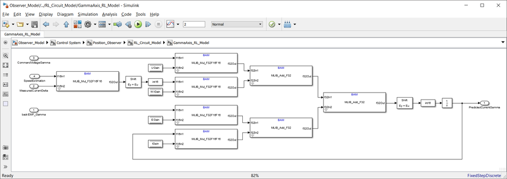
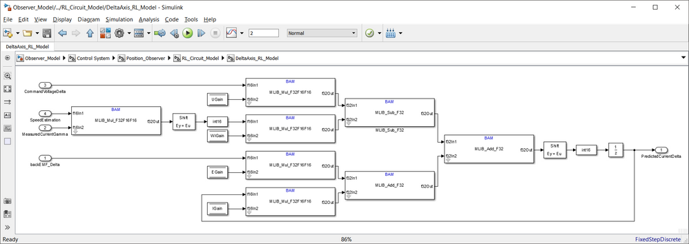
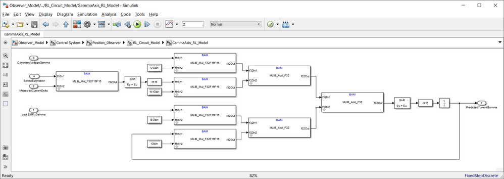
The Simulink model used to implement the Eq. 19 is shown below:
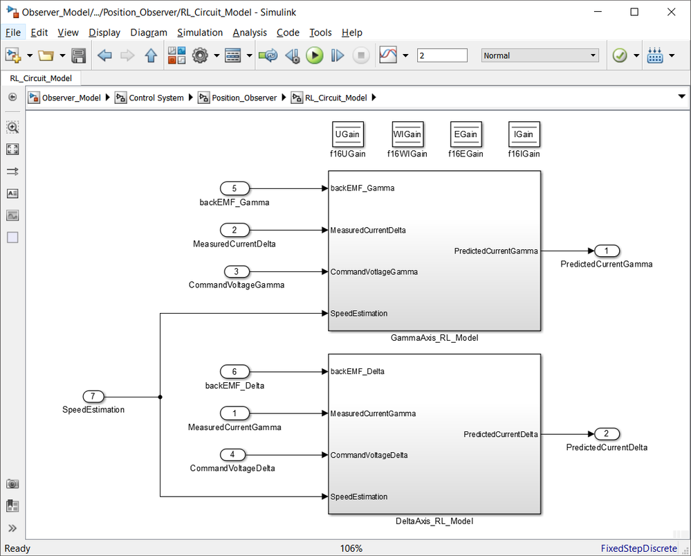 |
| Fig. 12: RL circuit implementation used to predict the current in γδ axes |
| Fig. 13: Implementation details for each of the gamma and delta axis based on Eq. 19 |
In order to check the accuracy of the predictions using this RL model lets compare the measured currents in dq frame with the predicted currents in γδ quasi-synchronous frame.
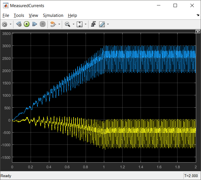 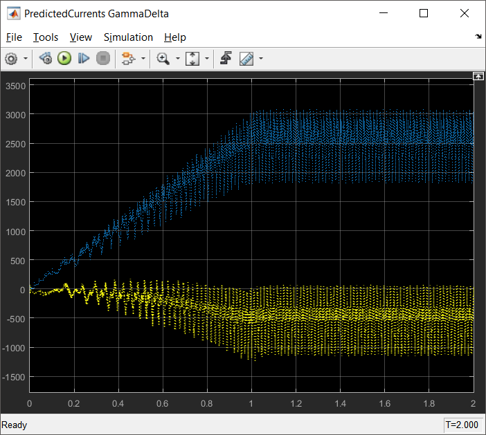 |
| Fig. 14: On the left hand side are the dq measured currents, while on the right hand side are the predicted currents using Eq. 19 |
At this point we have all the quantities we need to extract the rotor position information, therefore lets now talk about the actual back-EMF estimator.
2.3 back-EMF Estimator
The back-EMF estimator is formed in both of γδ axes and the resulting θerr is later on extracted from the division Eγ/Eδ. If we assume sufficient rotor speed to create back-EMF then, the result of the Eγ/Eδ division is insensitive to the actual level of back-EMF. This allows correct setup of the PI controllers.
The PI controllers (one for each of the gamma and delta axes) coefficients can be easy computed as shown before using the root-locus method. All you need to do is to set ξ (the current loop attenuation), and ω0 (the current loop natural frequency) and the easiest way for choosing those coefficients is to use same values chosen for the FOC current loop controllers.
The following code snipped can be used to compute automatically the controller parameters.
%%%%%%%%%%%%%%%%%%%%%%%%%%%%%%%%%%%%%%%%%%%%%%%%%%%%%%%%%%
% backEMF Observer parameters
%%%%%%%%%%%%%%%%%%%%%%%%%%%%%%%%%%%%%%%%%%%%%%%%%%%%%%%%%%
% (to be set according to the chosen control system dynamics)
Ts = 1e-4;              % sampling period [s]
i_Ksi = 1;              % current loop attenuation
i_fo = 300;             % current loop natural frequency [Hz]
i_wo = 2*pi*i_fo;       % current loop natural angular frequency [rad/s]
Kp = 2*i_Ksi*i_wo*Ld-Rs;
Ki = i_wo^2*Ld;

% PIr controller parameters for backEMF observers
maxCoeff = max(abs([( Kp + Ki*Ts/2)*Imax/Umax,...
    (-Kp + Ki*Ts/2)*Imax/Umax]));
NShift = max(0, ceil(log2(maxCoeff)));
if (NShift > 14)
    error('Inputted parameters cannot be used - u16NShift exceeds 14');
end

%f16CC1 for PIr backEMF controller in Gamma axis
PIr_BackEMF_Gamma_f16CC1 = (Kp + Ki*Ts/2)*Imax/Umax*2^-NShift;
PIr_BackEMF_Gamma_f16CC1 = round(PIr_BackEMF_Gamma_f16CC1 * 2^15);
PIr_BackEMF_Gamma_f16CC1(PIr_BackEMF_Gamma_f16CC1 < -(2^15)) = -(2^15);
PIr_BackEMF_Gamma_f16CC1(PIr_BackEMF_Gamma_f16CC1 > (2^15)-1) = (2^15)-1;

%f16CC2 for PIr backEMF controller in Gamma axis
PIr_BackEMF_Gamma_f16CC2 = (-Kp + Ki*Ts/2)*Imax/Umax*2^-NShift;
PIr_BackEMF_Gamma_f16CC2 = round(PIr_BackEMF_Gamma_f16CC2 * 2^15);
PIr_BackEMF_Gamma_f16CC2(PIr_BackEMF_Gamma_f16CC2 < -(2^15)) = -(2^15);
PIr_BackEMF_Gamma_f16CC2(PIr_BackEMF_Gamma_f16CC2 > (2^15)-1) = (2^15)-1;

%u16NShift for PIr backEMF controller in Gamma axis
PIr_BackEMF_Gamma_u16NShift = NShift;

%f16CC1 for PIr backEMF controller in Delta axis
PIr_BackEMF_Delta_f16CC1 = PIr_BackEMF_Gamma_f16CC1;
%f16CC2 for PIr backEMF controller in Delta axis
PIr_BackEMF_Delta_f16CC2 = PIr_BackEMF_Gamma_f16CC2;
%u16NShift for PIr backEMF controller in Delta axis
PIr_BackEMF_Delta_u16NShift = NShift;

disp(['PIr_BackEMF_Gamma_f16CC1 = ' num2str(PIr_BackEMF_Gamma_f16CC1) ';'])
disp(['PIr_BackEMF_Gamma_f16CC2 = ' num2str(PIr_BackEMF_Gamma_f16CC2) ';'])
disp(['PIr_BackEMF_Gamma_u16NShift = ' num2str(NShift) ';'])
disp(['PIr_BackEMF_Delta_f16CC1 = ' num2str(PIr_BackEMF_Delta_f16CC1) ';'])
disp(['PIr_BackEMF_Delta_f16CC2 = ' num2str(PIr_BackEMF_Delta_f16CC2) ';'])
disp(['PIr_BackEMF_Delta_u16NShift = ' num2str(NShift) ';'])
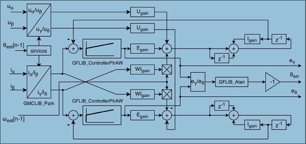
The Simulink model of the actual back-EMF estimator is shown in Fig. 15:
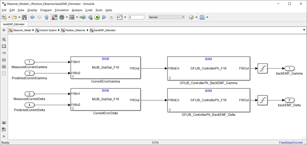 |
| Fig. 15: back-EMF estimator based on PI in recurrent form model |
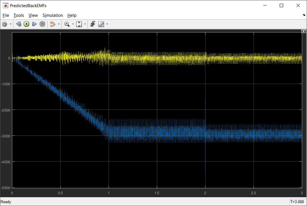
The outputs of the PI controllers represents the predicted back-EMF terms produced by rotating magnets in the motor stator coils and are shown in the Fig. 16:
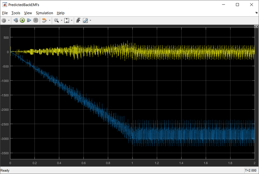 |
| Fig. 16: The back-EMF estimator predicted back-EMF waveforms for a speed profile with 1000rpm/sec ramp |
3. Position Tracking Observer
And finally we reached to the point where we can compute the actual rotor position and speed.
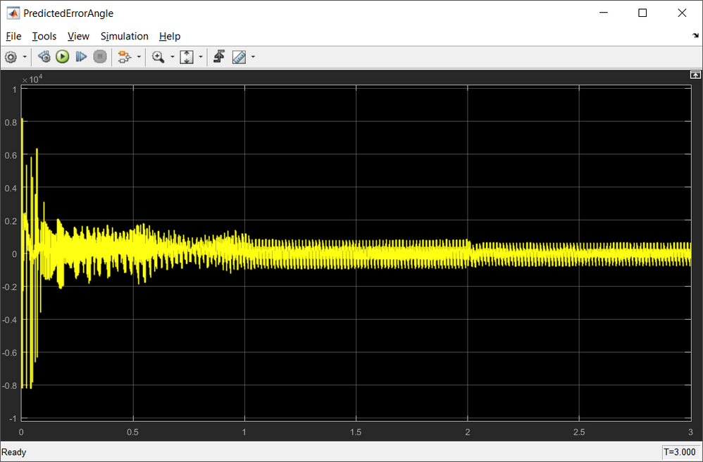
Since for the back-EMF estimator we have used the differences between the actual and estimated parameters, the resulting back-EMF estimates as outputs of PI controllers can be divided, to extract the information about the displacement between the estimated γδ and dq reference frames, while reducing the effect of the observer parameter variation. The position displacement θerr is obtained from Eq. 3.
The Simulink model used is shown in Fig. 17:
 |
| Fig. 17: θerr angle computation |
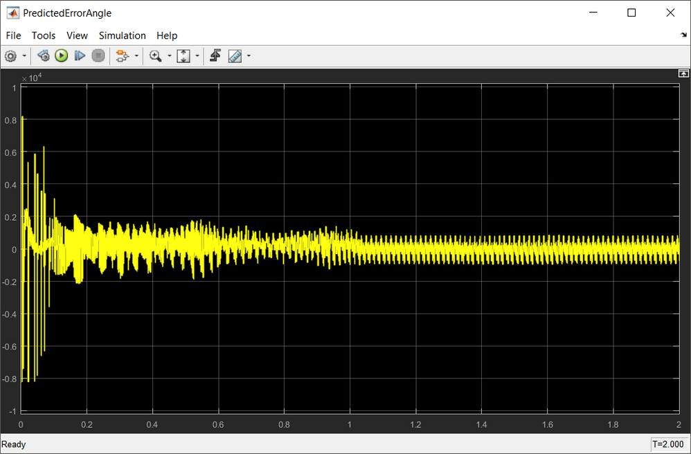 |
| Fig. 18: θerr angle variation during startup and steady state regime |
The rotor estimated position can then be obtained by driving the position of the estimated reference frame γδ, to achieve zero displacement θerr = 0. To achieve this, a phase locked loop mechanism is implemented, where the loop compensator ensures the correct tracking of the actual rotor position by trying to maintain the error signal θerr to zero.
The Simulink model of the position tracking observer with a standard PI controller used as the loop compensator is shown in Fig. 19:
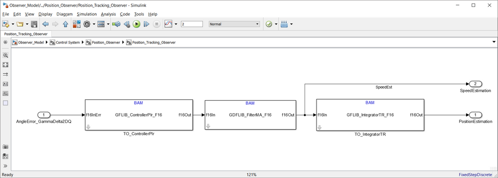 |
| Fig. 19: Position tracking observer based on PI controller |
As shown in Fig. 19, the position tracking controller consists of the standard PI controller and an Integrator. In between there is a moving average filter to level out some of the peaks within the estimated quantities.
Once again, using the root-locus tuning method we can compute the PI controller and Integrator gains starting from the second order characteristic polynomial. In this case the ξ is the required attenuation and the f0 is the required bandwidth of the position tracking loop. Since the position error signal is calculated by the back-EMF estimator formed in the rotating reference frame, the dynamics of the position tracking loop includes only frequencies proportional to the rate of change of rotor displacement which in general are lower than for the current loop.
Without going into many details about gains computations since these aspects were discussed in the beginning of this article, the following snipped can be used to compute automatically the position tracking observer parameters:
%%%%%%%%%%%%%%%%%%%%%%%%%%%%%%%%%%%%%%%%%%%%%%%%%%%%%%%%%%
% Tracking Observer parameters
%%%%%%%%%%%%%%%%%%%%%%%%%%%%%%%%%%%%%%%%%%%%%%%%%%%%%%%%%%
% (to be set according to the chosen control system dynamics)
p_Ksi = 0.707;          % position loop attenuation
p_fo = 15;              % position loop natural frequency [Hz]
p_wo = 2*pi*p_fo;       % position loop natural angular frequency [rad/s]
Kp = 4*pi*p_Ksi*p_fo;
Ki = p_wo^2;

% PIr controller parameters for position tracking observer
maxCoeff = max(abs([( Kp + (Ki*Ts)/2)*pi/Wmax,...
    (-Kp + (Ki*Ts)/2)*pi/Wmax]));
NShift = max(0, ceil(log2(maxCoeff)));
if (NShift > 14)
    error('Inputted parameters cannot be used - u16NShift exceeds 14');
end

%f16CC1 for PIr Tracking Observer controller
TO_ControllerPIr_f16CC1 = (Kp+(Ki*Ts)/2)*pi/Wmax*2^-NShift;
TO_ControllerPIr_f16CC1 = round(TO_ControllerPIr_f16CC1 * 2^15);
TO_ControllerPIr_f16CC1(TO_ControllerPIr_f16CC1 < -(2^15)) = -(2^15);
TO_ControllerPIr_f16CC1(TO_ControllerPIr_f16CC1 > (2^15)-1) = (2^15)-1;

%f16CC2 for PIr Tracking Observer controller
TO_ControllerPIr_f16CC2 = (-Kp+(Ki*Ts)/2)*pi/Wmax*2^-NShift;
TO_ControllerPIr_f16CC2 = round(TO_ControllerPIr_f16CC2 * 2^15);
TO_ControllerPIr_f16CC2(TO_ControllerPIr_f16CC2 < -(2^15)) = -(2^15);
TO_ControllerPIr_f16CC2(TO_ControllerPIr_f16CC2 > (2^15)-1) = (2^15)-1;

%u16NShift for PIr Tracking Observer controller
TO_ControllerPIr_u16NShift = NShift;

%f16C1, u16NShift for PIr Tracking Observer integrator
TO_IntegratorTR_f16C1 = (Ts/2)*Wmax/pi;
TO_IntegratorTR_f16C1 = round(TO_IntegratorTR_f16C1 * 2^15);
TO_IntegratorTR_u16NShift = 0;

disp(['TO_ControllerPIr_f16CC1 = ' num2str(TO_ControllerPIr_f16CC1) ';'])
disp(['TO_ControllerPIr_f16CC2 = ' num2str(TO_ControllerPIr_f16CC2) ';'])
disp(['TO_ControllerPIr_u16NShift = ' num2str(NShift) ';'])
disp(['TO_IntegratorTR_f16C1 = ' num2str(TO_IntegratorTR_f16C1) ';'])
disp(['TO_IntegratorTR_u16NShift = ' num2str(TO_IntegratorTR_u16NShift) ';'])
Now, if we run the model, we can get both the rotor position and speed.
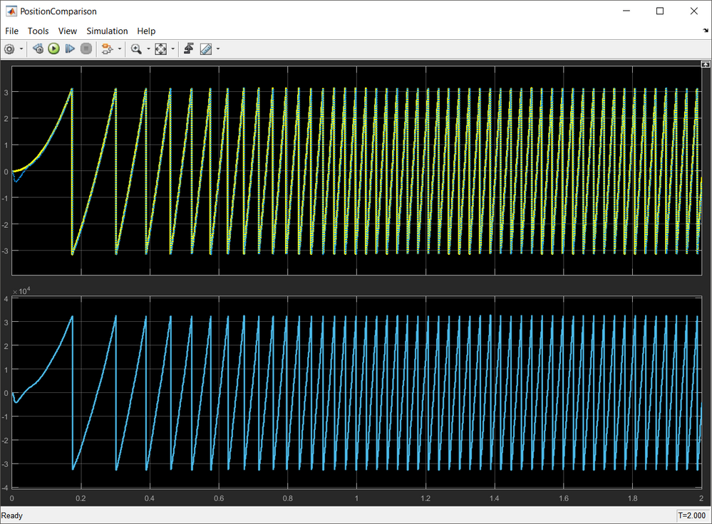 |
| Fig. 20: Predicted position (blue) against rotor true position (yellow). The predicted position is shown in both [rad] top, and scaled units [Q15] bottom |
 |
Fig. 21: Predicted position details: startup and delays (yellow - true rotor position, blue - predicted position using back-EMF estimator and Position Tracking Observer) |
In Fig. 22 is shown a comparison of the motor actual/true speed and the predicted value based on the position tracking observer output. As can be seen at startup the speed information is subject to error due to low back-EMF levels but once enough back-EMF is built into the motor coils the estimation becomes accurate. Fortunately we have the means to get rid of those errors by using the special startup sequence.
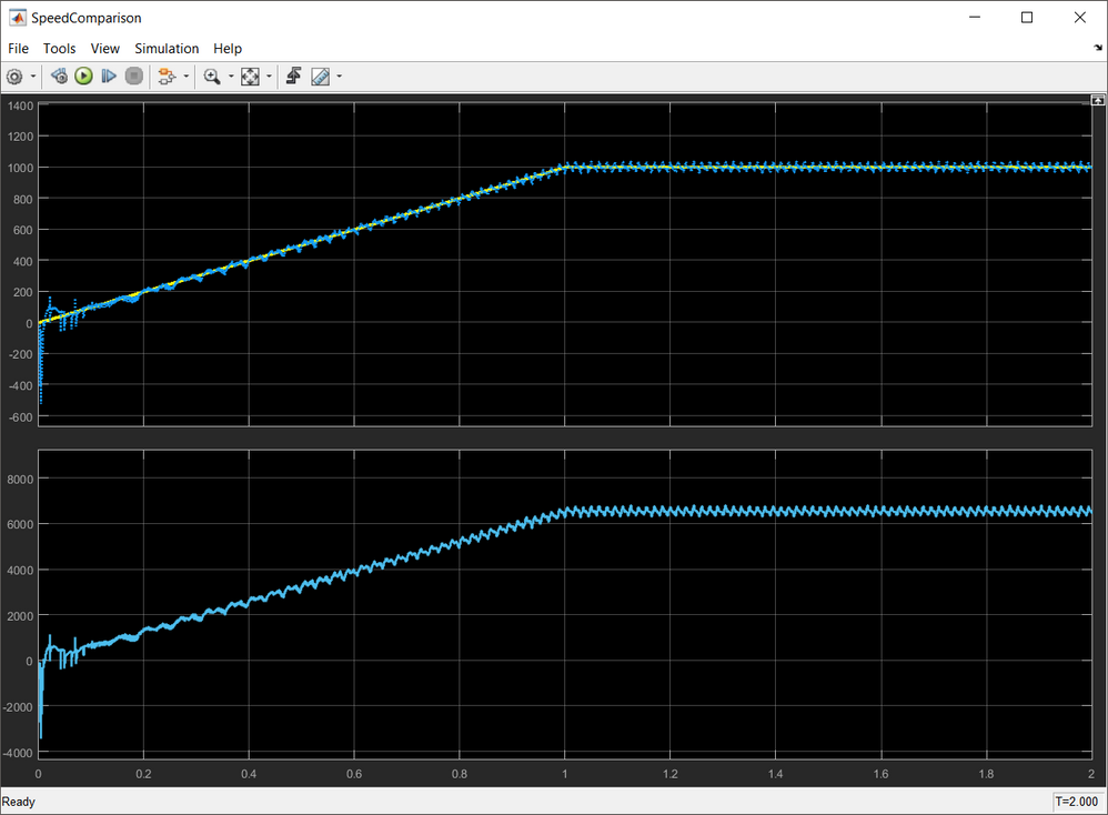 |
| Fig. 22: Rotor speed comparison: (yellow) true motor speed vs (blue) predicted speed |
EXPERIMENTS and VALIDATIONS
At this point we can say we have managed to build and tune a position observer using only standard blocks from AMMCLIB package. The main question that may arise now: can it handle motor parameter variations due to temperature changes ?
To check that, at 2 seconds after startup we are going to simulate an increase in motor phase resistance as is the motor copper coils have increased the temperature from 20 degC up to 100 degC
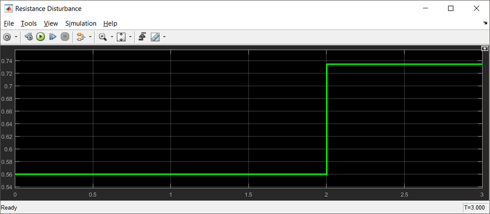 |
| Fig. 23: Disturbance due to phase resistance increase by 30% |
In this case the position observer predictions are:
| Fig. 24: Back-EMFs and Angle Error predictions in case of R increases suddenly by 30% |
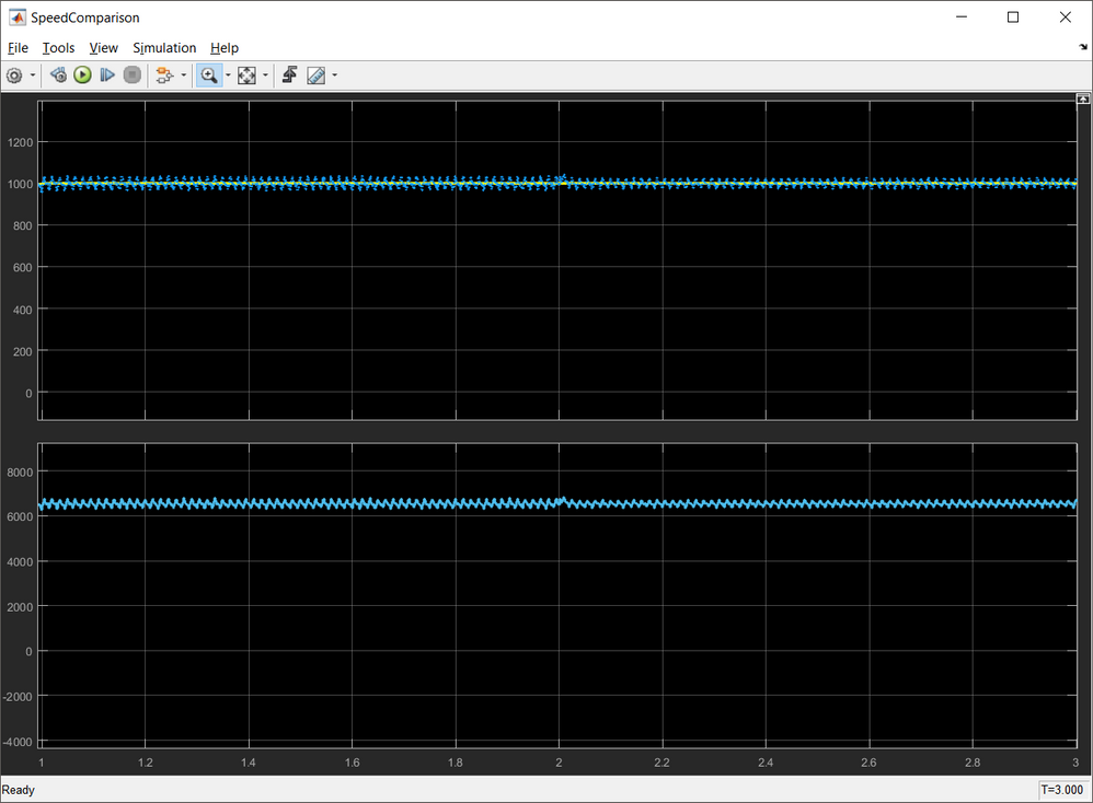
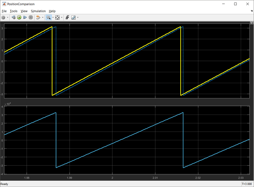
The only noticeable effect is small glitch in the estimated speed.
Fig. 25: Speed and Position prediction in case of R increases suddenly by 30%
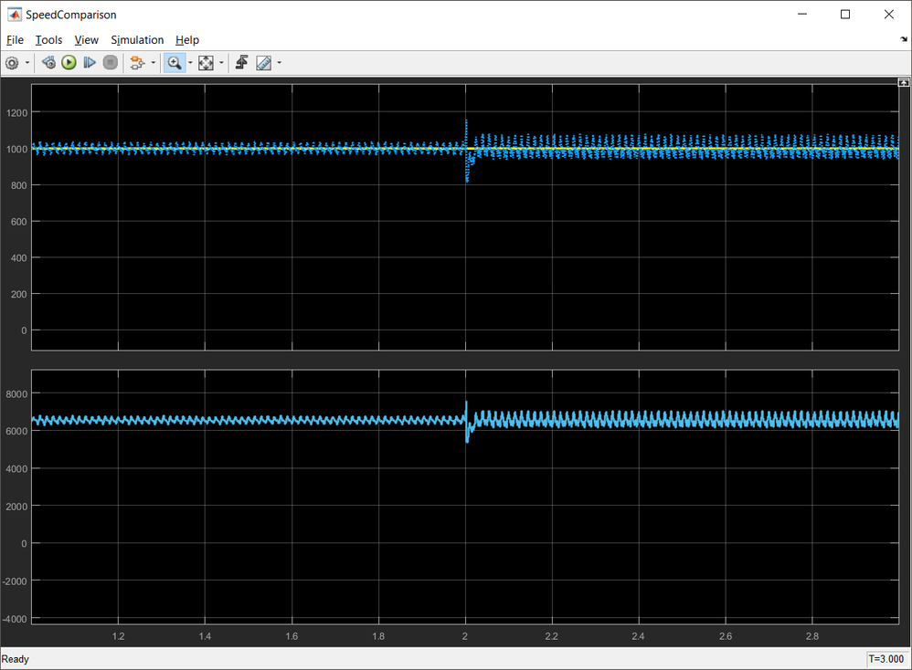
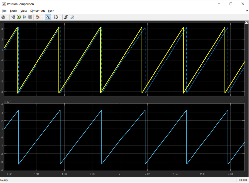
Now, let's assume that the R decreases by 50%:
| Fig. 26: Angle Error, Predicted Speed and Position in case of sudden decrease in R by 50% |
What other scenarios can you imagine for testing such position observer ?
CONCLUSIONS
Up to this point we have discussed the mathematical model and implementation of the position observer based on back-EMF estimation technique to predicts the rotor speed and position. We have checked its functionality in simulation environment to ensure the predictions are accurate against reference signals.
In the next module, we are going to integrate this position observer in the PMSM FOC system and used it to close the speed loop and get the rotor angle information required by PARK transformation.
Attached are the Simulink models and MATLAB scripts used in the module for designing the position observer.
Update January 28th 2019 - This Simulink model is now available on MATLAB 2018b and MBDT for S32K14x 2018.R1 release
Before using the new models make sure you apply all the hot-patches from here: HotFix: MBD Toolbox 2018.R1 for S32K
Update revisions:
March 18, 2019
- update the model to work with Model-Based Design Toolbox for MPC57xx Automotive Version 3.0.0 .
May 06, 2020
- update the model to work with Model-Based Design Toolbox for MPC57xx Automotive Version 3.2.0 .
- Mark as New
- Bookmark
- Subscribe
- Mute
- Subscribe to RSS Feed
- Permalink
- Report Inappropriate Content
thanks! that paper is very helpful。
I have a question.
the difference between the method "sliding mode" and "Position Observer". There are many articles using the method "sliding mode" without "Position Observer".
- Mark as New
- Bookmark
- Subscribe
- Mute
- Subscribe to RSS Feed
- Permalink
- Report Inappropriate Content
Thanks for the update and quick reply. I'll be sure to tellthebell keep an eye on this thread.
- Mark as New
- Bookmark
- Subscribe
- Mute
- Subscribe to RSS Feed
- Permalink
- Report Inappropriate Content
That’s what I was looking for, what a information! present MyMileStoneCard here at this website, thank you admin!!
- Mark as New
- Bookmark
- Subscribe
- Mute
- Subscribe to RSS Feed
- Permalink
- Report Inappropriate Content
Thank you for this extremely useful workshop! I have tried to implement the position observer in my project with S32K144, and it works perfectly with no load. However there seems to be a small estimation error that increases with current, resulting in step loss at high load. More specifically, the error seems to be approximately linearly dependent on both Iq and Id. Is this a known pheonomenon, or did I get something wrong with the implementation? Do you have any suggestion on how to fix it?
- Mark as New
- Bookmark
- Subscribe
- Mute
- Subscribe to RSS Feed
- Permalink
- Report Inappropriate Content
Hi Dainiel,
My matlab version is matlab 2019a and Model-Based Design Toolbox for S32K1xx Series Version 4.2.0.
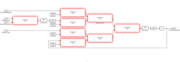
When I am opening the simulink model Observer_Model.mdl from M9_2018.R1 , all the libraries are showing as "unresolved link".
Could you please help me to resolve this issue.
- Mark as New
- Bookmark
- Subscribe
- Mute
- Subscribe to RSS Feed
- Permalink
- Report Inappropriate Content
Dear Daniel,
Thank you for a great workshop within this topic!
I have a couple of thoughts/questions that I would be glad if you cleared out to me!?
A. "If we rearrange the Eq. 18 in order to highlight...", shouldnt that be referring to Eq. 17 instead?
B. When looking at your implementation of Eq 19 in the simulink environment I get insecure.
B0. As people are asking about where the (k-1) variables disappears I guess that the variable is
considered to be fairly constant from one sample to another? But then there should be a *2 in there too, shouldn't it?
B1. The "Shift Ey = Eu" blocks, what is that?
B2. Shouldn't the output of the "PredictedCurrentGamma" be routed from before the 1/z block?
C. Under the section when you calculate the parameters for the Back-emf controllers. Can you please tell what PIr_BackEMF_Gamma_f16CC1 and PIr_BackEMF_Gamma_f16CC2 are? Are these the proportional and integrating controller amplificatons?
Hope you can help out!
Best regards,
Tomas
- Mark as New
- Bookmark
- Subscribe
- Mute
- Subscribe to RSS Feed
- Permalink
- Report Inappropriate Content
Hi,Daniel
In the Eq.19, we have to add E(k-1)、W(k-1)*I(k-1)、U(k-1),
but in the RL_Circuit_Model block, we no need to add this, I have a doubt about it , thanks you!
Best regards,
- Mark as New
- Bookmark
- Subscribe
- Mute
- Subscribe to RSS Feed
- Permalink
- Report Inappropriate Content
Daniel,
I would like to know the answer on this question as well.
- Mark as New
- Bookmark
- Subscribe
- Mute
- Subscribe to RSS Feed
- Permalink
- Report Inappropriate Content
Sorry for delay! For some reasons i was not aware of these replies.
First of all, thank you all for highlighting this issue. I think you are right.
The correct implementation should be something like this:
I'm going to recheck the model in the next days and i'll let you know my finding.
In any case if anyone of you have already fix the model and is willing to share it - i would be more than happy to reuse it.
Best regards,
Daniel
- Mark as New
- Bookmark
- Subscribe
- Mute
- Subscribe to RSS Feed
- Permalink
- Report Inappropriate Content
Hi dumitru-daniel.popa,
I have modelled the back-EMF observer using the block diagram you posted (which can be also found in the AMMCLIB user guide) and I can confirm that it works. However, could you please share for reference a link or article which details how the difference equations are derived?
Regards,
Luca
- Mark as New
- Bookmark
- Subscribe
- Mute
- Subscribe to RSS Feed
- Permalink
- Report Inappropriate Content
Hi Luca,
Did you got any reference which details how the differential equations are derived? If yes, could you please share it...Thanks in Advance
Regards
AJ
- Mark as New
- Bookmark
- Subscribe
- Mute
- Subscribe to RSS Feed
- Permalink
- Report Inappropriate Content
这个问题你搞懂了吗?
- Mark as New
- Bookmark
- Subscribe
- Mute
- Subscribe to RSS Feed
- Permalink
- Report Inappropriate Content
I have the same problem
- Mark as New
- Bookmark
- Subscribe
- Mute
- Subscribe to RSS Feed
- Permalink
- Report Inappropriate Content
Hello Daniel,
I read your topic in another link, that is about PMSM VF control, Thanks for your wonderful teaching.
But I have a boubt, PMSM its modle under open-loop is unstable, from small signal modling and its root locus,we can see it may have unstable poles when rotor speed changes. So Is it necessary to add a stable loop while using VF control?I know some approach about adding stable loop for PMSM-VF driving.
Here is one of them:A sensorless, stable V/f control method for permanent-magnet synchronous motor drives - IEEE Journal... . It takes a high pass filter to abstract the ripple of the rotor speed from motor power and compensates it. (P=U*I*Powerfactor)
Because I have a SPMSM, but I need to control it under low speed, and BEMF estimation doesn't work for low speed operation. Moreover, High frequency signal injection method will not work as well due to Ld=Lq.(Sensorless FOC)
Hmm~~
No position sensor, no available parameters estimator, So it reminds me of VF control. Could you please give me some advice?
Thank you
ZiJun.Wan
2018.9.28
- Mark as New
- Bookmark
- Subscribe
- Mute
- Subscribe to RSS Feed
- Permalink
- Report Inappropriate Content
i am from china。
Position Observer (Part 1/2):question about Eq1,Eq2。
how these eq1,eq2 come from?
can you give me some book name about that? thanks。
- Mark as New
- Bookmark
- Subscribe
- Mute
- Subscribe to RSS Feed
- Permalink
- Report Inappropriate Content
Hi wu chao,
There are many articles and books available for free on the internet. I can't indicate a specific book but the eq. 1 and 2 represent the PMSM mathematical model in fixed orthogonal system (alpha/beta) which is standard.
Anyhow, please find here attached a generic article about PMSM equations. Have a look at eq. 1-7 (page 9). It is the same with eq. 1 with the following assumptions:
- v0 = 0 due to the motor symetrie
- rs = R
- Lls+3/2Lms = L
- p (Laplace operator) = d/dt
lapbda*dOr/dt =kv*w
Hope this helps!
Daniel
- Mark as New
- Bookmark
- Subscribe
- Mute
- Subscribe to RSS Feed
- Permalink
- Report Inappropriate Content
thanks! that paper is very helpful。
now i have another question: how to determine Q-aligned or D-aligned to a sensorless motor?
Sincerely
wuchao
sdust
