- Forums
- Product Forums
- General Purpose MicrocontrollersGeneral Purpose Microcontrollers
- i.MX Forumsi.MX Forums
- QorIQ Processing PlatformsQorIQ Processing Platforms
- Identification and SecurityIdentification and Security
- Power ManagementPower Management
- Wireless ConnectivityWireless Connectivity
- RFID / NFCRFID / NFC
- Advanced AnalogAdvanced Analog
- MCX Microcontrollers
- S32G
- S32K
- S32V
- MPC5xxx
- Other NXP Products
- S12 / MagniV Microcontrollers
- Powertrain and Electrification Analog Drivers
- Sensors
- Vybrid Processors
- Digital Signal Controllers
- 8-bit Microcontrollers
- ColdFire/68K Microcontrollers and Processors
- PowerQUICC Processors
- OSBDM and TBDML
- S32M
- S32Z/E
-
- Solution Forums
- Software Forums
- MCUXpresso Software and ToolsMCUXpresso Software and Tools
- CodeWarriorCodeWarrior
- MQX Software SolutionsMQX Software Solutions
- Model-Based Design Toolbox (MBDT)Model-Based Design Toolbox (MBDT)
- FreeMASTER
- eIQ Machine Learning Software
- Embedded Software and Tools Clinic
- S32 SDK
- S32 Design Studio
- GUI Guider
- Zephyr Project
- Voice Technology
- Application Software Packs
- Secure Provisioning SDK (SPSDK)
- Processor Expert Software
- Generative AI & LLMs
-
- Topics
- Mobile Robotics - Drones and RoversMobile Robotics - Drones and Rovers
- NXP Training ContentNXP Training Content
- University ProgramsUniversity Programs
- Rapid IoT
- NXP Designs
- SafeAssure-Community
- OSS Security & Maintenance
- Using Our Community
-
- Cloud Lab Forums
-
- Knowledge Bases
- ARM Microcontrollers
- i.MX Processors
- Identification and Security
- Model-Based Design Toolbox (MBDT)
- QorIQ Processing Platforms
- S32 Automotive Processing Platform
- Wireless Connectivity
- CodeWarrior
- MCUXpresso Suite of Software and Tools
- MQX Software Solutions
- RFID / NFC
- Advanced Analog
-
- NXP Tech Blogs
- Home
- :
- Model-Based Design Toolbox (MBDT)
- :
- Model-Based Design Toolbox (MBDT)
- :
- Module 9: Position Observer (Part 1/2)
Module 9: Position Observer (Part 1/2)
- Subscribe to RSS Feed
- Mark Topic as New
- Mark Topic as Read
- Float this Topic for Current User
- Bookmark
- Subscribe
- Mute
- Printer Friendly Page
Module 9: Position Observer (Part 1/2)
- Mark as New
- Bookmark
- Subscribe
- Mute
- Subscribe to RSS Feed
- Permalink
- Report Inappropriate Content
 |
INTRODUCTION
As we have discussed in the previous modules of the 3-Phase PMSM Control Workshop with NXP's Model-Based Design Toolbox, to control a PMSM optimally, the position or the speed of the rotor must be known. In general the rotor position/speed is measured using a position transducer like hall sensors or dedicated sensors like encoders/resolvers. By knowing the rotor position and by maintaining a correct angle between the stator and rotor magnetic fluxes, the PMSM can be controlled in such a way that it provides full torque at zero speed.
Nonetheless, the presence of such position sensors in PMSM control systems is usually undesirable due to:
- increases the cost and the complexity of the overall control system (drive, motor, sensors, maintenance)
- increased number of connections between the motor and the drive system
- electromagnetic interference due to the presence of connecting leads
- limited measuring accuracy due to environmental factors such as temperature, humidity and vibrations
To address these problems highlighted above, researchers proposed the sensor-less control of PMSM. The basic idea behind this concept is to get rid of the position sensors by trying to determine the actual rotor position indirectly by measuring other variables such as motor's voltages and currents. The term sensor-less control means that there is no position/speed sensors used but there are sensors which measure the currents.
SENSOR-LESS METHODS
In the technical literature there are a lot of sensor-less control strategies each of them having its own advantages, disadvantages and limitations but if we try to classify these methods we will end up with two major classes:
- PMSM model based methods: as the name implies these methods are based on the electrical model of PMSM, and are known to achieve good results in medium and high-speed operation. Due to these limitations the model based methods are mainly used in low-end applications
- Methods based on PMSM magnetic saliency: are using the magnetic saliency (Ld is different than Lq) inherent characteristic of PMSM. Such methods are known to achieve good results in standstill or very low speed region and are mainly used for certain type of PMSM motors designed accordingly
i. Back-EMF Based Methods
This method uses the PMSM inherited relationship between the back-EMF and rotor position. This method is based on the PMSM mathematical model and uses the stator currents and voltages of the PMSM to compute the back-EMF space vector in order to get the rotor angle.
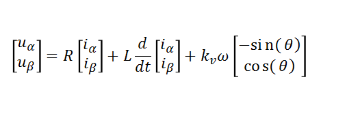
Because the rotor permanent magnet flux is aligned with the d-axis (one of FOC goals), the back-EMF is always placed on the q-axis. The rotor position can be calculated by projecting the back-EMF vector from the dq-axes on the stationary orthogonal reference frame αβ as shown in Eq. 1 which represent the PMSM mathematical model.
|
Eq. 1
Eq. 2 |
Using Eq. 2 we can simply compute the PMSM rotor position as:
 |
Eq. 3 |
Based on this basic mathematical model there are many other back-EMF based methods which relies on the use of flux Observers or Kalman filters with the whole purpose to improve the estimation procedure and algorithm stability. Such methods can give good results in the medium and high speed operating region while at low speed rand standstill due to lack of back-EMF produces as consequence of small speed the estimation becomes problematic. The main limitation of the back-EMF based methods is that it can not be used for sensor-less control of a PMSM in the zero and low speed region (less that 5% rates speed).
Since the measured phased currents are used for back-EMF calculation makes these methods prone to noise influence while the overall accuracy is affected by the motor parameters R, L, flux constant that might vary with the temperature.
ii. Stator Flux Linkage Based Methods
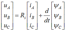
Another way of estimating the PMSM rotor position is to make use of the stator flux linkage vector. The PMSM stator flux linkage vector is calculated using the rotor reference frame dq voltage equations as shown by Eq. 4:
 |
Eq. 4 |
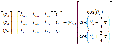
The flux equations used above are:
 |
Eq. 5 |
For more details about these equations please check: Module 2: PMSM and FOC Theory
Similar with the computations made for the back-EMF method, the Eq. 5 can be projected from the dq-axes on the stationary orthogonal reference frame αβ as shown in Eq. 6
|
Eq. 6 |
As you can see the phase voltages, currents and resistance must be measured and known in order to calculate the stator fluxes and ultimately the rotor position.
The main issue with this method is cause by the integration processes that might drift over time. Of course we may get rid of this problem by using proper integration methods but still the main limitation as shown for back-EMF remains - the initial rotor position is not detectable with this sensor-less technique.
iii. Inductance Based Methods
This class of methods are based on the fact that PMSM stator phase inductances are dependent of rotor position, thus an observer could be built to track the variation of the phase inductance over an electrical period.
where: |
Eq. 7 |
Usually such sensor-less techniques will obtain the rotor position information from on-line calculation of the stator phase inductances which are compared against a look-up table which contains a given inductance for a given rotor position. Such methods relies on the knowledge of stator resistance and PM flux linkage values. In addition a high switching frequency ( >10kHz) is needed for inductance calculations.
By itself such method is not suitable to determine the rotor position at zero speed since the phase voltages are closed to zero at standstill and is very susceptible to error caused by certain parameter variations.
iIV. Observers Based Methods
Such techniques are using various forms of the PMSM mathematical model which are used to create a virtual system that is excited with the same phase voltages as the actual system. The goal is to have this virtual model to produce estimated outputs, which are then compared with the measured outputs of the real motor. The errors between the virtual and the physical quantities are used to correct the outputs of the state observer which is then used to correct the PMSM rotor position.
Nonetheless, since the PMSM model is nonlinear by definition, the design and implementation of a state observer is generally quite complex but the algorithms may often be very robust against parameter variations and measurement noise. The main drawbacks of this approach is highly computational requirements and design complexity. In addition to all these the observer based methods can not detect initial rotor position.
iV. Signal Injection Based Methods
These methods are using a high frequency signal that is superimposed on top of the fundamental phase voltage that controls the PMSM. This high frequency signal induces currents which contain information about the rotor position that can be decoded via specialized signal processing techniques.
Such techniques are especially used for sensor-less control of salient pole or interior magnets PMSM types due their high saliency ratio. However, the same technique can be used with surface mounted PMSM since it is going to exploit the saliency produced by the saturation effect of the stator core due to the rotor permanent magnet flux.
For the PMSM the magnetic reactance in the d-axis is lower than the one in the q-axis. This is why the magnitude of the current measured in d-axis is higher than the one measured in the q-axis for the same injection voltage signal. The opposite is true for the inductance in the d-axis is lower than the inductance in the q-axis. This effect is caused by the saturation of the magnetic core around d-axis. Based on these observations an accurate observer could be built to harness the effect of magnetic saturation and accurately estimate the speed even at zero speed.
SELECTION OF POSITION ESTIMATION METHOD
(Proof-of-Concept)
Based on the general description of the available methods suitable for sensor-less control methods shown above, it seems that saliency based methods like high frequency signal injection might be the best way to estimate the rotor position due to ability to work even at standstill conditions. However, since they are only well-suited for motors with inductance variations over one electrical period, in case of small motors with surface mounted magnets that have negligible dq saliency, the resulting variations in the measured currents would be too low to produce a proper position estimation. In our particular case, due to commutation noises it will be almost impossible to distinguish the phase current variations due to magnetic saturation.
That being said, we have practically only type of sensor-less method left. Overall, the back-EMF-based methods are quite popular and suitable for the proposed control system. The limitation to provide accurate position estimation at low speeds is not a problem, since at low-speed operation we can use the open loop voltage control.
Therefore, let us see how can we build a simple back-EMF estimator.
In order to understand the concept let us start from a simple use case such as a PMSM with surface mounted permanent magnets that is assumed to have no saliency (Ld = Lq) as the one described by Eq. 2. The representation of the mathematical model (basically the CLARKE coordinate transformation from 3 phase machine into 2 phase orthogonal) for the phase windings is shown in Fig. 1.
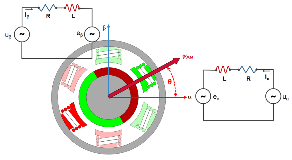 |
| Fig. 1: PMSM stator model in αβ stationary orthogonal reference frame |
These two windings (sine and cosine) are placed at 90 electrical degrees one of each other and from Eq. 2 we can clearly see that the rotor angle θ is in direct relationship with the two back-EMF voltages eα and eβ.
So, if we find a way to evaluate these back-EMF voltages, then we can simply apply the Eq. 3 and get the rotor angle. Piece of cake, right ?
Measuring the back-EMF is impossible when using FOC since all phases are commutated at all time, therefore the only viable option is to find a numerical method to extract the back-EMF information from the mathematical model.
As a side note, in case of BLDC 6-step commutation method where at any moment in time only 2 out of 3 motor phases are energized, it is possible to measure the back-EMF of the un-connected phase, but that is a topic for another discussion.
If we look closely at the winding model and assume there are no AC values but rather only DC quantities, then that looks exactly like a DC motor model which is much more simple to simulate and understand. So, let us see how can we can build a basic back-EMF estimator starting from the DC motor model. First we need to write the Kirchhoff circuit law for one of the windings shown in Fig. 1 (e.g.: for the sine winding along alpha axis) the equation becomes:
|
Eq. 8 |
The Eq. 8 shows that the voltage applied to any of the motor coils (e.g. uα) is equal to the sum of the voltages around the loop: voltage drop due to coil resistance and inductance and the back-EMF generated inside the coil due to rotor spinning magnets eα. What is interesting about this equation, is that the rotor position θ is embedded inside the back-EMF voltage term. Finding a way to estimate the back-EMF will allow us to know the rotor position.
From mathematical point of view, we can estimate the back-EMF term with a simple observer that is based on the applied voltage uα, the measured current iα and the motor winding parameters R & L.
We can build this back-EMF observer starting from the current that flows thru the coil. From Eq. 8 we can derived the estimated current as:
 | Eq. 9 |
Note that current, resistance and inductance in Eq. 9 are marked with the hat operator since all these are predicted values.Now comes the really interesting part: if we can make the predicted current from Eq. 9 to be equal with the measured current from Eq. 8 then we can have a very good guess of what the back-EMF term is. This equality can only happen if the predicted back-EMF is equal with the real back-EMF generated inside the motor windings.
Fortunately, is quite easy to build such an observer in the Simulink environment using the Eg. 9 and the model below:
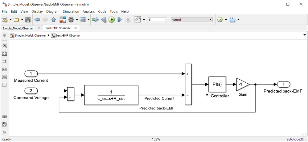 |
| Fig. 2: Simplified back-EMF observer model |
As can be seen in Fig. 2, the predicted current is computed based on the difference between the command voltage, the predicted back-EMF and some estimated values for the motor winding resistance and inductance values. Then, the predicted current is compared against the motor phase measured current and the difference is fed into a PI controller that has the job to minimize the error between these 2 currents. If the error is kept to zero by this PI controller then it means that the output of the controller is the exact back-EMF that is produced inside the motor coil. The negative gain is added to stabilize the closed loop around the PI controller.
If we run the simulation and compare the actual back-EMF of a DC motor against the predicted back-EMF we can check how the observer behaves.
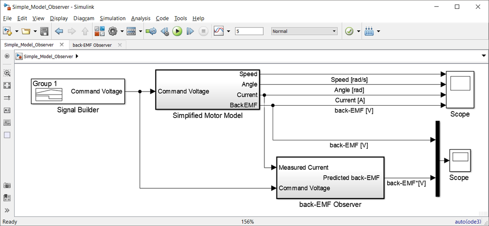 |
| Fig. 3: Simulink model to simulate the motor and back-EMF observer operations |
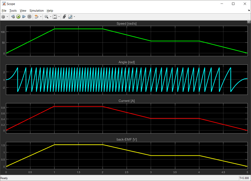
As shown in Fig. 4, the motor is supplied with a variable voltage pattern that cause it to speed up and down to certain levels and than back to stall. The motor simplified model is used to check the rotor position, motor current and phase winding back-EMF that are used as references for the back-EMF observer.
 |
| Fig. 4: Simplified motor model outcome waveforms used as references |
The back-EMF observer output, the predicted back-EMF, is shown in the Fig. 5 and compared with the motor back-EMF obtained from simplified motor model. As can be seen, the observer can predict quite accurately the back-EMF. The accuracy of the back-EMF observer is tightly coupled with the PI controller gains. In theory, the PI controller should be able to deal with R variations due to temperature changes.
 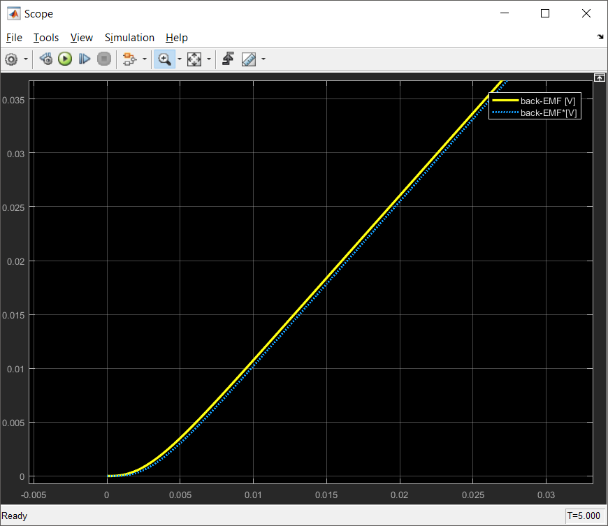 |
| Fig. 5: Predicted back-EMF (dotted-blue) vs. actual motor back-EMF (solid-yellow) comparison |
The PI controller within the back-EMF observer can be tuned based on root-locus method as any of PI standard current controller. Starting from Eq. 9, we can depict the process transfer function as a standard 1st order transfer function:
where: |
Eq. 10 |
The PI controller, assuming the parallel form can be written as:
where: Kp and Ki are the proportional and integral controller gains, respectively |
Eq. 11 |
 |
| Fig. 6: Generic closed loop system derived from model shown in Fig. 2 |
Using the Eq. 10 and Eq. 11 we can write the transfer function of the closed loop system shown in Fig. 6, from the motor measured current to the predicted current as:
 |
Eq. 12 |
Now, if we identify each coefficient from the closed loop system characteristic polynomial against the standard second order system desired response (Eq. 13) we can compute the actual values of the PI controller gains:
 | Eq. 13 |
More information about root-locus tuning method and PI controllers can be found here: Motor Control Class: Lecture 11 - Closed Loop Control
The values of the PI controller that predicts the missing back-EMF term from Eq. 8 are:
Eq. 14 |
This is how you can build a simple observer using the measured current and command voltage to predict the variation of the back-EMF voltage. At this point we only have one of the back-EMF waveform. Now, we need to find the other back-EMF waveform that corresponds to the orthogonal axis and then using the Eq. 3, to evaluate the rotor position.
So, if up to this point you found this article interesting, lets dig more into the problem an see how can we build a control system around back-EMF observers.
POSITION OBSERVER
Most likely this is one of the most complex subjects we are going to tackle in this workshop. The complexity is derived mainly from the mathematical background required to implement such task but also due to the nature of PMSM that requires a good knowledge of the machine operation, magnetic field decoupling and modelling.
Also, in order to address some of the concerns raised by different users within this community, to keep the implementation as generic as possible in order to work with other MCU, we are going to use 16 bit fixed point implementation using only common blocks from AMMCLIB that are available across all the other toolboxes.
Due to the subject complexity this chapter is devided in 3 main topics in order to allow readers to understand the specific aspects without losing the focus on the big picture:
- Theory of operation - how it works and the mathematical background;
- Back-EMF Estimator - implementation of the R-L circuit that predicts the currents and PI back-EMF controller tuning;
- Position Tracking Observer - why is important to minimize the tracking error and how to tune the PI tracking controller;
1. Theory of operation
When we discuss about the position observer within a Field Oriented Control system we are referring at 3 major computation blocks that are required to predict the PMSM rotor position as depicted in the Fig. 7
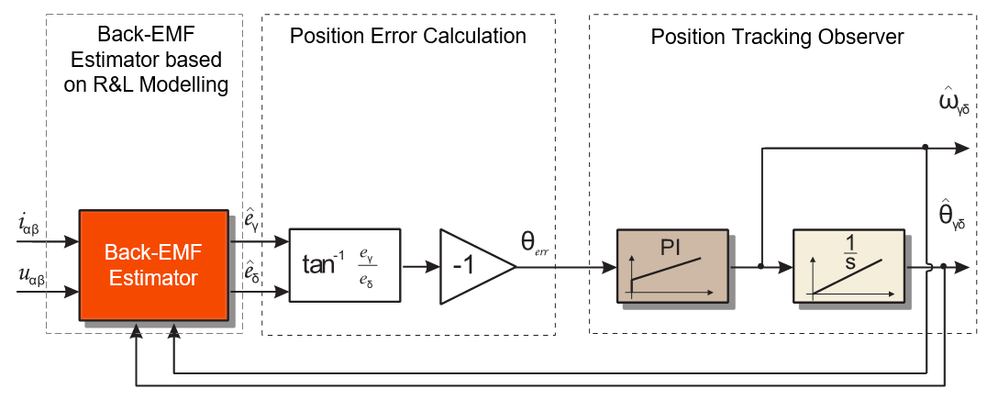 |
| Fig. 7: Block diagram of the Position Estimator |
For modelling, we are going to use a slightly different implementation than the one described in the previous chapter and the reason will become evident in a moment. The back-EMF estimator we are going to use is going to estimate the saliency based back-EMF which is predicted with a PI controller.
For that we are going to consider a new orthogonal virtual frame γδ - gamma/delta which is a rotating coordinate system synchronous with the rotating magnetic field produced in the PMSM. This virtual γδ - gamma/delta frame has the same properties as the standard dq - direct/quadrature coordinate system used for the torque and flux decoupling equations in FOC (check Module 2: PMSM and FOC Theory for more information) but compared with that one is offset by an error angle θerr as shown in Fig. 8 .
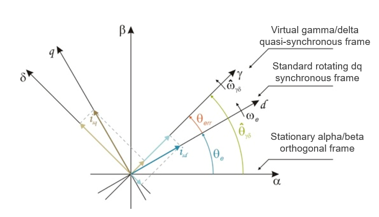 |
| Fig. 8: PMSM rotor and stator reference frames |
So, why do we need this new frame γδ - gamma/delta ?
Well, now comes one of the most important technical aspects of the theory behind this position observer. If you look closely at the frames depicted in Fig. 8, something interesting happens if γδ is perfectly aligned with dq frame. If the error angle θerr is zero than all the saliency back-EMF, generated by the rotating magnets, is located in the δ-delta axis which is in fact same as the q axis and this means that there is no error between real and estimated position. This is the quintessence of the whole position estimation mechanism.
On the other hand, if error angle θerr exists then, the γ-gamma axis also see saliency back-EMF, therefore the back-EMF voltage can be our cost-function that needs to be optimized towards zero by help of a simple PI controller.
Therefore, from now on we are going to use this γδ - gamma/delta frame to perform all the computations related to position observer. Considering the Eq.1, we can rewrite the PMSM model in the γδ - gamma/delta as:
 |
Eq. 15 |
where:
- R is the resistance of one stator phase [Ω],
- Ld and Lq are the d-axis and q-axis inductances [H],
- ωγδ is the estimated electrical angular velocity of the rotor [rad/s],
- uγ and uδ are the stator voltages [V],
- iγ and iδ are the stator currents [A],
- kv*ωγδ is the saliency-based BEMF magnitude [V],
- θerr is the phase error between the estimated quasi-synchronous frame γδ and the synchronous rotor flux frame dq [rad],
- s is the Laplace differential operator.
Please note that in Eq. 15, the voltage in the δ-axis is computed from the Ld inductance instead of Lq. This helps us to avoid the motor parameters measurement errors of the R and Ld parameters. This is yet another reason for selecting this implementation of saliency based back-EMF since position estimation accuracy depends only on one parameter until the field weakening region. The only parameter that needs to be known/measured beforehand is Lq. All other model based approaches methods depends on 2 or 3 of the motor parameters (Rs,Ld,Lq)
Information about how to measure various motor parameters can be found here
So the output of the back-EMF estimator are the saliency back-EMF voltages in γδ error frame and we already know that we need to optimize the γ-gamma component to be zero or better to say the angle error θerr between γδ error frame and the dq frame to be zero.
As shown in Fig. 7, with the help of tangent function we can obtain directly the angle error θerr between γδ error frame and the dq frame which can be directly optimized to zero by a third PI controller (the first two of PI controller are inside the back-EMF estimator). This PI controller is part of what we call a Position Tracking Observer.
If the angle error θerr between γδ error frame and the dq frame is zero then we also have the correct position on the output of the Position Tracking Observer and on the output of PI controller there must be the correct speed.
The overall Simulink model for the Position Observer based on the components we have discussed in this sub-chapter is shown in Fig. 9.
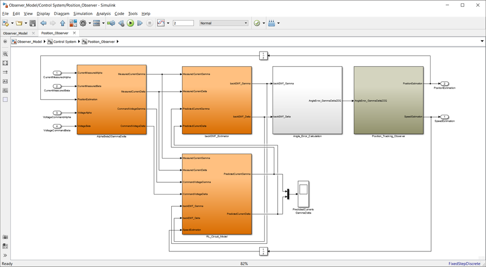 |
| Fig. 9: Simulink model of the Position Estimator for FOC of PMSM |
2. back-EMF Estimator
The back-EMF estimator (others might call it back-EMF observer but for the sake of avoiding term overlapping with Position Observer, i'll refer to it as estimator) job is to detect the voltages induced by the permanent magnets of a PMSM in this newly introduced quasi-synchronous γδ reference frame. The estimated back-EMF quantities allows the estimation of the rotor speed and position.
As depicted in Fig. 9 with orange blocks, for readability I broke the back-EMF estimator into 3 Simulink subsystems:
- AlphaBeta2GammaDelta subsystem projects the real current and voltages into the quasi-synchronous frame
- RL_Circuit_Model subsystem implements the PMSM model that is used to predict the currents in the quasi-synchronous frame
- backEMF_Estimator implements the PI controllers that computes the back-EMF quatities in the quasi-synchronous frame
2.1 αβ2γδ Transformations
The input voltages and currents are supplied in a stationary reference frame αβ. The back-EMF estimator, transforms these quantities into a quasi-synchronous reference frame γδ that follows the real synchronous rotor flux frame dq with an error θerr. These transformations are shown in Fig. 10, and as can be seen this is nothing more that a simple PARK transformation in which the angle used for sine/cosine computations is the one predicted by the Position Observer
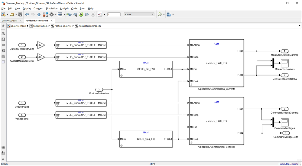 |
| Fig. 10: AlphaBeta to GammaDelta coordinate transformation Simulink model |
Also, please note that all the inputs are converted from floating point single precision to fixed point 16 bit numbers using dedicate AMMCLIB conversion block. In case of the current we also need to scale the values to (-1, 1) interval using a simple divide with the ADC maximum measurable current value. As shown in Fig. 11, even if we changed the numeric representation the currents and voltages continue to have the variation we expect from a FOC. The scaling factor is easy to be deducted is we consider that at 2^15 we get the maximum current of 31.25Amps or maximum voltage of 12Volts.
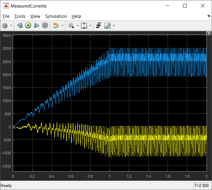 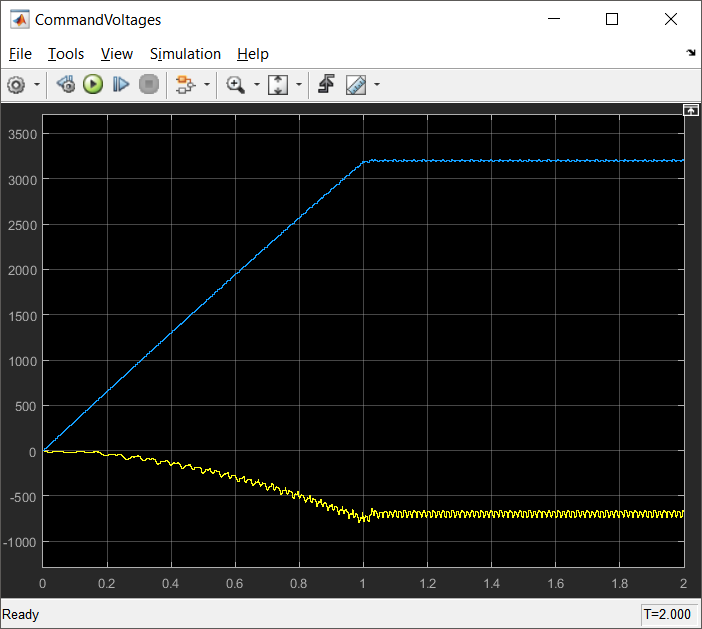 |
Fig. 11: Currents and Voltage in γδ quasi-synchronous frame after αβ2γδ transformation, assuming a trapezoidal speed profile with a slope of 1000rpm/sec |
For the moment please ignore the noisiness of the measured currents. This is due the simplified model used for PMSM windings
The part 2/2 of this article can be found here: https://community.nxp.com/message/1020634
- Mark as New
- Bookmark
- Subscribe
- Mute
- Subscribe to RSS Feed
- Permalink
- Report Inappropriate Content
https://www.nxp.com/webapp/sps/download/preDownload.jsp?render=true that link is empty.
can you give another link or give the document file name ,so i can find in internet by myself.
thanks.
- Mark as New
- Bookmark
- Subscribe
- Mute
- Subscribe to RSS Feed
- Permalink
- Report Inappropriate Content
in Eq. 5 at Module 9: Position Observer (Part 1/2),i think ω*φd is missing in φα,either for φβ。am i wrong?
and as for:As shown in Fig. 4, the motor is supplied with a variable voltage pattern that cause it to speed up and down to certain levels and than back to stall.---------------it seems "than back to stall"is wrong for "then back to stall".
and as for:
if up to this point you found this article interesting, lets dig more into the problem an see-------is ' and see' right?
by the way your article is very interesting and helpful! thanks
- Mark as New
- Bookmark
- Subscribe
- Mute
- Subscribe to RSS Feed
- Permalink
- Report Inappropriate Content
Hi carlwu,
Sorry for delay - for some reasons i'm not getting updates to all thread that happens on this community and some of the replies might be overlooked.
As shown in Fig. 4, the motor is supplied with a variable voltage pattern that cause it to speed up and down to certain levels and than back to stall.---------------it seems "than back to stall"is wrong for "then back to stall".
The figure shows the Electric Angle, Current and Back-EMF when the motor is accelerated up to 1000rpm in 1sec, then is keeping that speed for another 1sec followed by a 1sec deceleration ramp to 500 rpm, maintaining 500rpm for another second and then decelerated to 0 or stall.
in Eq. 5 at Module 9: Position Observer (Part 1/2),i think ω*φd is missing in φα,either for φβ。am i wrong?
Eq. 5 is written in DQ reference frame hence there should be no αβ components.
In general, i've used this document as reference: https://www.nxp.com/webapp/sps/download/preDownload.jsp?render=true and other equation that can be found on the web.
Hope this helps!
Daniel
- Mark as New
- Bookmark
- Subscribe
- Mute
- Subscribe to RSS Feed
- Permalink
- Report Inappropriate Content
Hi Daniel,
Thank you very much for the interesting posting, it is very inspiring!
The link you shared in the reply to wu chao does not seem to work - it just directs to the Software Center and no download starts.
Could you please reshare?
Thanks a lot,
Radek
