- Forums
- Product Forums
- General Purpose MicrocontrollersGeneral Purpose Microcontrollers
- i.MX Forumsi.MX Forums
- QorIQ Processing PlatformsQorIQ Processing Platforms
- Identification and SecurityIdentification and Security
- Power ManagementPower Management
- Wireless ConnectivityWireless Connectivity
- RFID / NFCRFID / NFC
- Advanced AnalogAdvanced Analog
- MCX Microcontrollers
- S32G
- S32K
- S32V
- MPC5xxx
- Other NXP Products
- S12 / MagniV Microcontrollers
- Powertrain and Electrification Analog Drivers
- Sensors
- Vybrid Processors
- Digital Signal Controllers
- 8-bit Microcontrollers
- ColdFire/68K Microcontrollers and Processors
- PowerQUICC Processors
- OSBDM and TBDML
- S32M
- S32Z/E
-
- Solution Forums
- Software Forums
- MCUXpresso Software and ToolsMCUXpresso Software and Tools
- CodeWarriorCodeWarrior
- MQX Software SolutionsMQX Software Solutions
- Model-Based Design Toolbox (MBDT)Model-Based Design Toolbox (MBDT)
- FreeMASTER
- eIQ Machine Learning Software
- Embedded Software and Tools Clinic
- S32 SDK
- S32 Design Studio
- GUI Guider
- Zephyr Project
- Voice Technology
- Application Software Packs
- Secure Provisioning SDK (SPSDK)
- Processor Expert Software
- Generative AI & LLMs
-
- Topics
- Mobile Robotics - Drones and RoversMobile Robotics - Drones and Rovers
- NXP Training ContentNXP Training Content
- University ProgramsUniversity Programs
- Rapid IoT
- NXP Designs
- SafeAssure-Community
- OSS Security & Maintenance
- Using Our Community
-
- Cloud Lab Forums
-
- Knowledge Bases
- ARM Microcontrollers
- i.MX Processors
- Identification and Security
- Model-Based Design Toolbox (MBDT)
- QorIQ Processing Platforms
- S32 Automotive Processing Platform
- Wireless Connectivity
- CodeWarrior
- MCUXpresso Suite of Software and Tools
- MQX Software Solutions
- RFID / NFC
- Advanced Analog
-
- NXP Tech Blogs
- Home
- :
- モデルベース・デザイン・ツールボックス(MBDT)
- :
- NXP モデルベースデザインツール for VISION ナレッジベース
- :
- AI and Machine Learning Course #5: Transfer Learning with NXP Vision Toolbox on S32V
AI and Machine Learning Course #5: Transfer Learning with NXP Vision Toolbox on S32V
- RSS フィードを購読する
- 新着としてマーク
- 既読としてマーク
- ブックマーク
- 購読
- 印刷用ページ
- 不適切なコンテンツを報告
AI and Machine Learning Course #5: Transfer Learning with NXP Vision Toolbox on S32V
AI and Machine Learning Course #5: Transfer Learning with NXP Vision Toolbox on S32V
In this 5th module of the AI and Machine Learning with S32V and MATLAB - Workshop we are going to discuss the following topics:
- How to retrain a CNN in MATLAB
- How to run custom CNN on the NXP S32V microprocessor
- Brief introduction to training your own model from scratch
1. INTRODUCTION
In practice, very few people train an entire Convolutional Neural Network from scratch (with random initialization), because it is relatively rare to have a dataset of sufficient size. Instead, it is common to pretrain a CNNon a very large dataset (e.g. ImageNet, which contains 1.2 million images with 1000 categories), and then use the CNN either as an initialization or a fixed feature extractor for the task of interest.
Transfer learning involves the approach in which knowledge learned in one or more source tasks is transferred and used to improve the learning of a related target task. While most machine learning algorithms are designed to address single tasks, the development of algorithms that facilitate transfer learning is a topic of ongoing interest in the machine-learning community. Transfer learning is commonly used in deep learning applications. You can take a pretrained network and use it as a starting point to learn a new task. Fine-tuning a network with transfer learning is usually much faster and easier than training a network with randomly initialized weights from scratch.
You can quickly transfer learned features to a new task using a smaller number of training images.
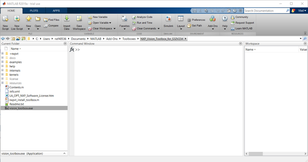
To get all of the files needed by the example in the tutorial you should run the vision_toolbox.exe archive in the root of the Vision Toolbox as in the window below and overwrite all files that the prompt asks you about:
You can also find the training set attached (the four .7z archives). They contain all the 64 classes used for training in this tutorial.
2. CUSTOMIZING THE MODEL
This tutorial was done using MATLAB R2018b. The R2019a release introduces a couple of changes that will require some porting work. As soon as we update the toolbox to use the new version of MATLAB, we will update the tutorial as well.
In order to retrain the model using an already trained network as a starting point, one can tweak the network's layers, augment the training dataset, change some of the learning parameters or other use some of the fine-tuning techniques out there. We are going to showcase the toolbox's capabilities with one example that is not yet available in the toolbox, but that will get posted here. We are going to be talking about a Traffic Sign Recognition system using the Belgian traffic signs database which one can obtain by downloading from the training data from https://btsd.ethz.ch/shareddata/BelgiumTSC/BelgiumTSC_Training.zip and the testing data from https://btsd.ethz.ch/shareddata/BelgiumTSC/BelgiumTSC_Testing.zip.
2.1 CONFIGURING THE DATASET
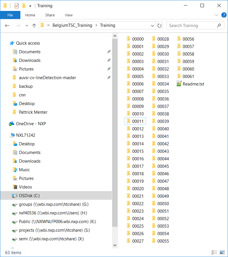
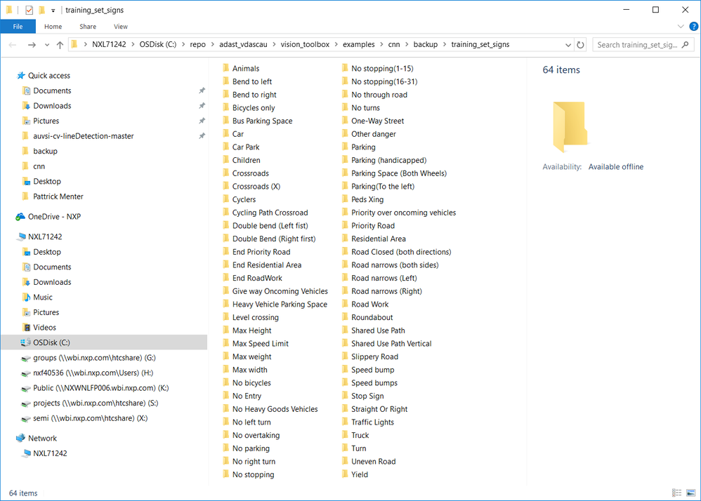
After downloading the dataset, we have renamed all the folders to the class they represent (traffic sign name). The raw data is divided into 62 classes (00000 - 00061) :
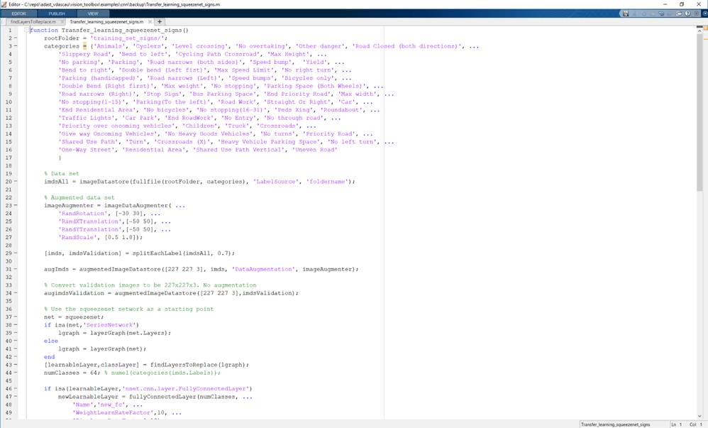
As you can see we have also added the Cars and Trucks folder with our own data. First thing we need to do is to actually set the class names in a variable called categories that will hold the names of all folders in the training_set_signs folder.
2.2 AUGMENTING THE DATASET
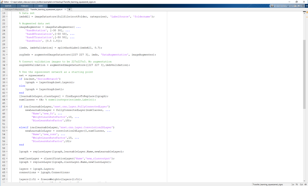
Before actually diving into (re)training a CNN, MATLAB provides a way to increase the input dataset on the fly, preventing over-fitting and allowing users to get the most of their data. Over-fitting occurs when you achieve a good fit of your model on the training data, while it does not generalize well on new, unseen data. In other words, the model learned patterns specific to the training data, which are irrelevant in other data.
In MATLAB, this step only boils down to configuring a set of preprocessing options for augmenting the image, using a special object. An augmented image datastore transforms batches of training, validation, test, and prediction data, with optional preprocessing such as resizing, rotation, and reflection. It also allows resizing the available images to make them compatible with the input size of the deep learning network. For a complete overview of MATLAB's capabilities regarding this subject, visit https://www.mathworks.com/help/deeplearning/ug/preprocess-images-for-deep-learning.html#mw_ef499675-... .
Augmenting the data in our example consists of applying:
- random rotations ( -30 degrees to 30 degrees )
- random X and Y translations ( -50 to +50 pixels )
- scaling/zooming ( 0.5 to 1.8).
The datastore automatically resizes the input images to 227x227x3, which is the format that SqueezeNet was trained on and the only image format it accepts:
2.3 REPLACING CLASSIFICATION LAYERS
Going forward, we should first understand the layers of the SqueezeNet network.
The convolutional layers of the network extract image features that the last learnable layer and the final classification layer use to classify the input image. These 2 layers (learnable and classification) contain information on how to combine the features that the network extracts into class probabilities, a loss value, and predicted labels.
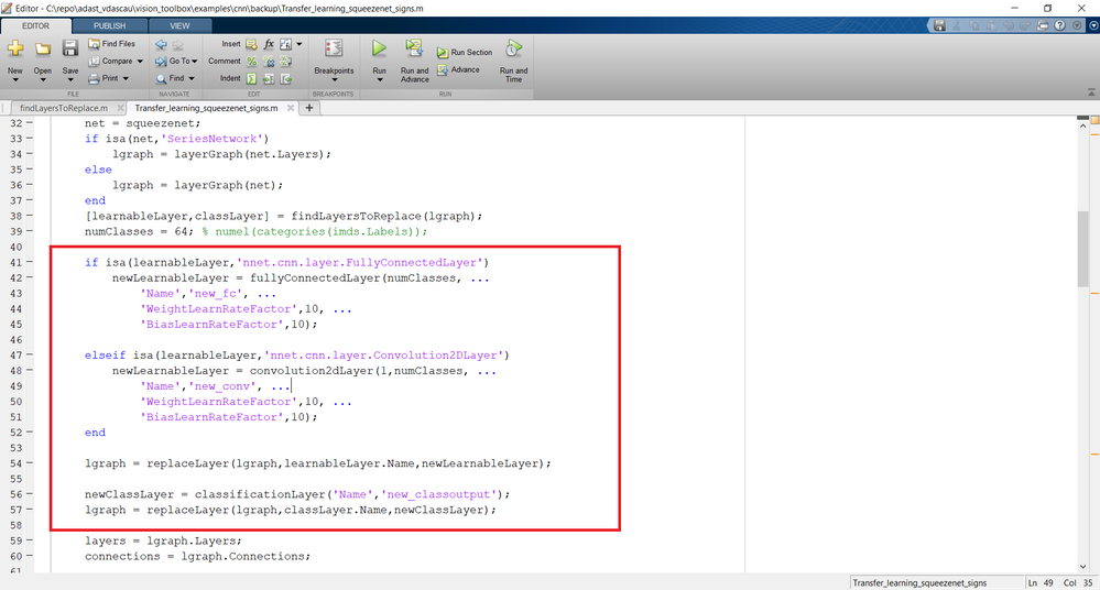
To retrain a pretrained network to classify new images, we need to replace these two layers with new layers adapted to the new data set. We first extract the layer graph from the trained network. If the network is a SeriesNetwork object, such as AlexNet, VGG-16, or VGG-19, then the list of layers in net.Layers to a layer graph gets converted into a LayerGraph.
In most networks, the last layer with learnable weights is a fully connected layer. Replace this fully connected layer with a new fully connected layer with the number of outputs equal to the number of classes in the new data set (5, in this example). In some networks, such as SqueezeNet, the last learnable layer is a 1-by-1 convolutional layer instead. In this case, replace the convolutional layer with a new convolutional layer with the number of filters equal to the number of classes. To learn faster in the new layer than in the transferred layers, increase the learning rate factors of the layer.
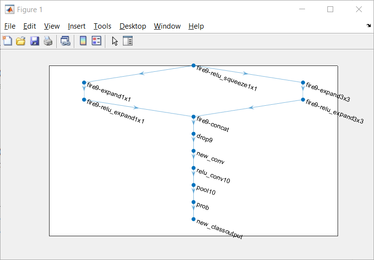
Finding the layers to be replaced is done with the helper function findLayersToReplace which is provided by MATLAB in one of their example. You can find it attached here if you want to understand more on how it is used to determine the layers that have to get replaced. The classification layer specifies the output classes of the network, thus we have to replace the classification layer with a new one without class labels. The trainNetwork function automatically sets the output classes of the layer at training time. To check that the new layers are connected correctly, we can plot the new layer graph and zoom in on the last layers of the network:
The network is now ready to be retrained on the new set of images. Optionally, you can "freeze" the weights of earlier layers in the network by setting the learning rates in those layers to zero. During training, the trainNetwork function does not update the parameters of the frozen layers. Because the gradients of the frozen layers do not need to be computed, freezing the weights of many initial layers can significantly speed up network training. If the new data set is small, then freezing earlier network layers can also prevent those layers from over-fitting to the new data set.
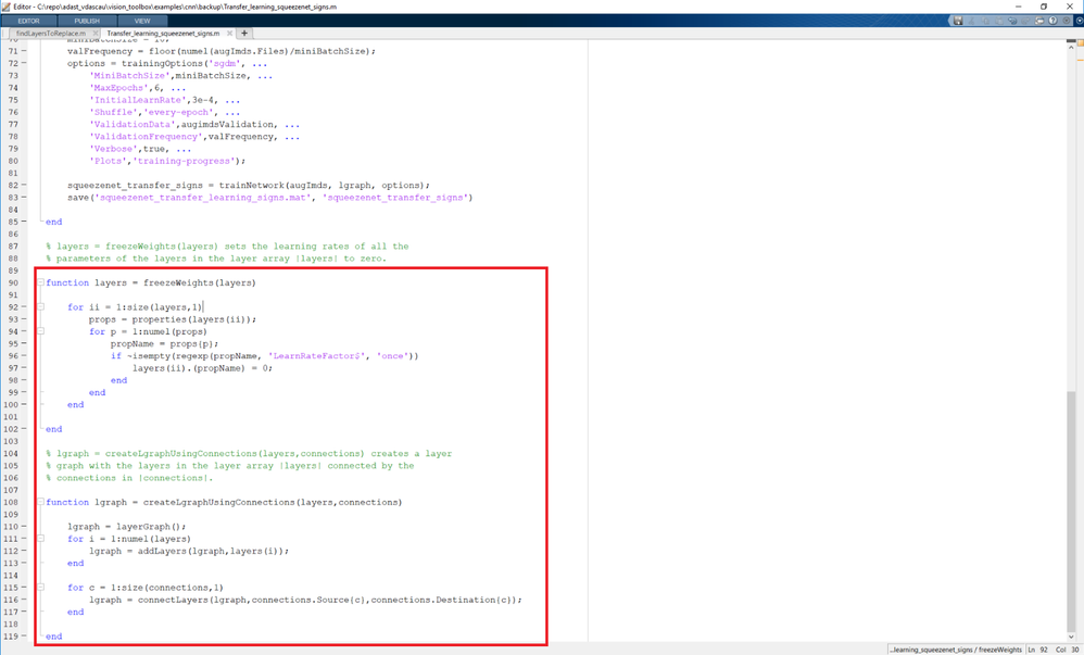
Extract the layers and connections of the layer graph and select which layers to freeze. We will make use of the supporting function createLgraphUsingConnections to reconnect all the layers in the original order. The new layer graph contains the same layers, but with the learning rates of the earlier layers set to zero:
3. RETRAINING THE MODEL
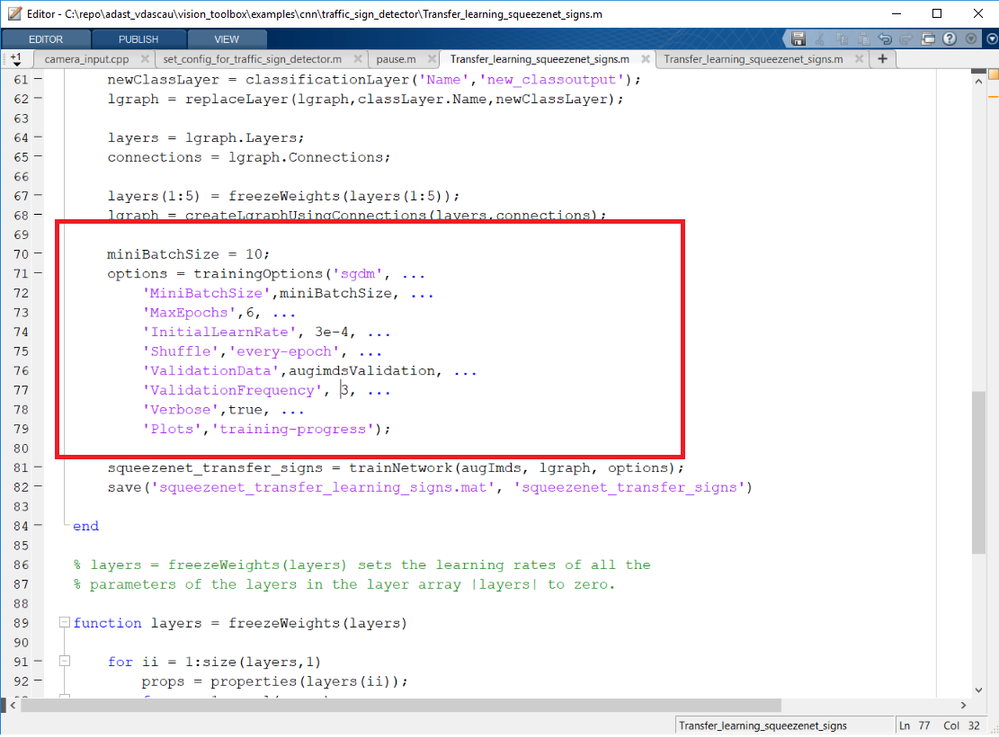
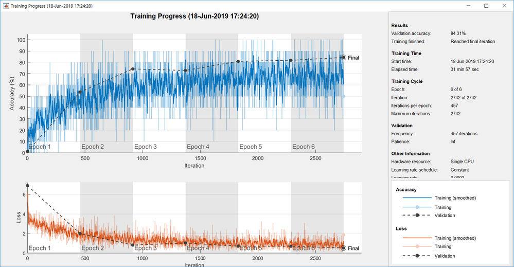
The actual training is done is the next code snippet. We provide the training options in a trainingOptions structure with a set of parameters ( which, by the way, can be tweaked in an attempt to increase accuracy ). We are using SGDM ( Stochastic Gradient Descent with Momentum ) optimizer, mini-batches with 10 observations at each iteration, an Initial learning rate of 0.0003 and a total of 6 epochs for the training process. Training with this parameters took 32 minutes with a Single CPU hardware resource and achieved a pretty decent 84% validation accuracy level.The training duration can be dramatically improved by using a GPU and the Parallel Computing Toolbox from MATLAB.
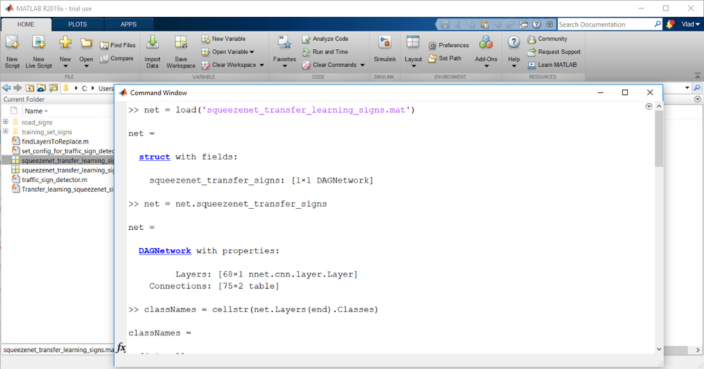
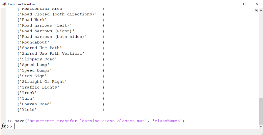
Last thing we want to do before actually testing all the work we've done is to save the classNames for the generated CNN:
At this point you should be ready to test the network, if all went according to the plan.
4. TESTING THE CUSTOMIZED NETWORK
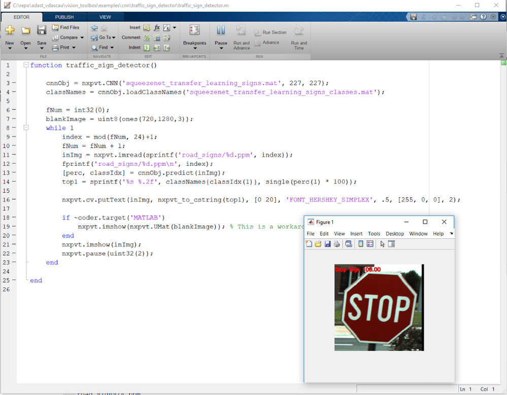
After training the script saves the new trained network in a .mat file, which should be then loaded using the same manner show in the previous courses. You should run the self-extracting archive in the toolbox's root to get a hold of the files in the example. To run the traffic sign detector example, just run the traffic_sign_detector() script.
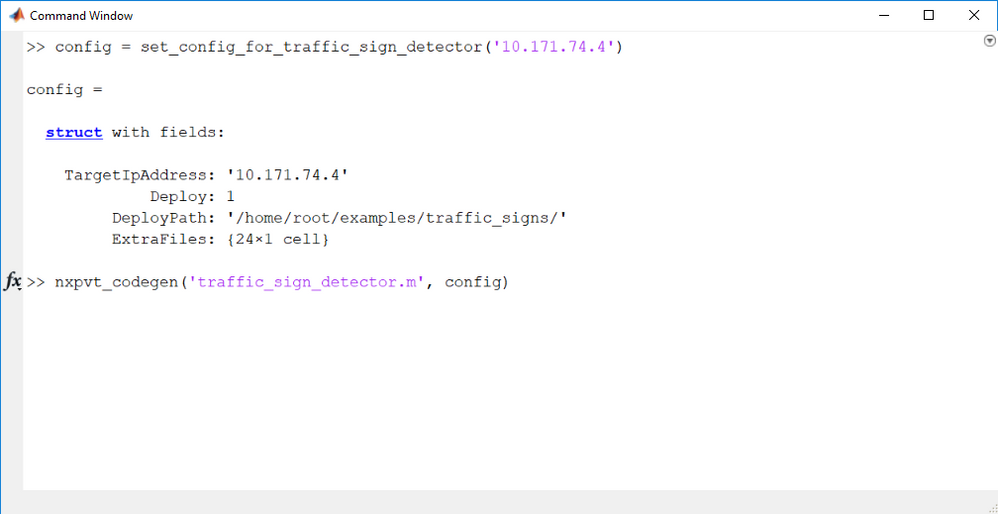
To run it on the target board, you should copy the input images to the board. To do that, you can use the helper set_config_for_traffic_sign_detector.m :
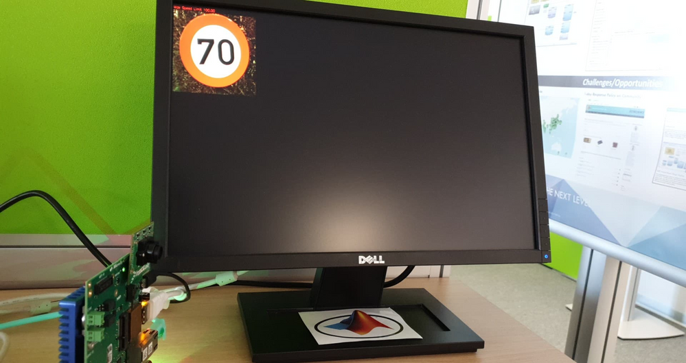
You now should be getting the expected results from the board:
5. CONCLUSIONS AND FURTHER WORK
The NXP Vision Toolbox represents a flexible addition that enables users to get things up and running in no time, and allows deployment of algorithms on the NXP boards bringing the MATLAB world into the embedded one.
It combines the versatility of MATLAB with the rapidity of the NXP boards by harnessing all the power the hardware accelerators provide. On top of that it allows Convolutional Neural Networks deployment. Additional ongoing development is happening to accelerate the neural networks (by running the computation-intensive neural network on APEX accelerators) with an internal engine that is also under development. Stay tunes for updates in the near future.
- 既読としてマーク
- 新着としてマーク
- ブックマーク
- ハイライト
- 印刷
- 不適切なコンテンツを報告
Very good, practical material which should speed up one's intro into CNN
