- NXP Forums
- Product Forums
- General Purpose MicrocontrollersGeneral Purpose Microcontrollers
- i.MX Forumsi.MX Forums
- QorIQ Processing PlatformsQorIQ Processing Platforms
- Identification and SecurityIdentification and Security
- Power ManagementPower Management
- MCX Microcontrollers
- S32G
- S32K
- S32V
- MPC5xxx
- Other NXP Products
- Wireless Connectivity
- S12 / MagniV Microcontrollers
- Powertrain and Electrification Analog Drivers
- Sensors
- Vybrid Processors
- Digital Signal Controllers
- 8-bit Microcontrollers
- ColdFire/68K Microcontrollers and Processors
- PowerQUICC Processors
- OSBDM and TBDML
-
- Solution Forums
- Software Forums
- MCUXpresso Software and ToolsMCUXpresso Software and Tools
- CodeWarriorCodeWarrior
- MQX Software SolutionsMQX Software Solutions
- Model-Based Design Toolbox (MBDT)Model-Based Design Toolbox (MBDT)
- FreeMASTER
- eIQ Machine Learning Software
- Embedded Software and Tools Clinic
- S32 SDK
- S32 Design Studio
- Vigiles
- GUI Guider
- Zephyr Project
- Voice Technology
- Application Software Packs
- Secure Provisioning SDK (SPSDK)
- Processor Expert Software
-
- Topics
- Mobile Robotics - Drones and RoversMobile Robotics - Drones and Rovers
- NXP Training ContentNXP Training Content
- University ProgramsUniversity Programs
- Rapid IoT
- NXP Designs
- SafeAssure-Community
- OSS Security & Maintenance
- Using Our Community
-
- Cloud Lab Forums
-
LPC55S69 + PowerQuad Part 3 : Fast Fourier Transforms - Rulers, Gauges and Protractors
LPC55S69 + PowerQuad Part 3 : Fast Fourier Transforms - Rulers, Gauges and Protractors
- Subscribe to RSS Feed
- Mark as New
- Mark as Read
- Bookmark
- Subscribe
- Printer Friendly Page
- Report Inappropriate Content
In my last article, we examined a common time domain filter called the Biquad and how it could be computed using the LPC55S69 PowerQuad engine. We will now turn our attention to another powerful component of the PowerQuad, the “Transform Engine”. The PowerQuad transform engine can compute a Fast Fourier Transform (FFT) in both a power and time efficient manner leaving your main CPU cores to handle other tasks.
Before we look at the implementation on the LPC55S69, I want to illustrate what exactly an FFT does to a signal. The meaning of the data is often glossed over or even worse yet, explained in purely mathematical terms without a description of *context*. I often hear descriptions like “transform a signal from the time domain to the frequency domain”. While these types of descriptions are accurate, I think that many do not get an intuitive feel for what the numbers are *mean*. I remember my 1st course in ordinary differential equations. The professor was explaining the Laplace transform (which is more generalize case of the Fourier Transform) and I asked the question “What does s actually mean in a practical use case?”.
Figure 1. Laplace Transform. What is s?
My professor was a brilliant mathematician and a specialist in complex analysis. He could explain the transform from 3 different perspectives with complete mathematical rigor. Eventually we both got frustrated and he said “s will be a large number complex number in engineering applications”. It turned out the answer was simple in terms of the electrical engineering problems we were solving. After many years and using Laplace again in Acoustic Grad School it made sense but at the time it was magical. I hope to approach the FFT a bit differently and you will see it is simpler than you may think. While I cannot address all the aspect of using FFT’s in this article, I hope it gives you a different perspective from a “getting started” perspective.
Rulers, Protractors, and Gauges
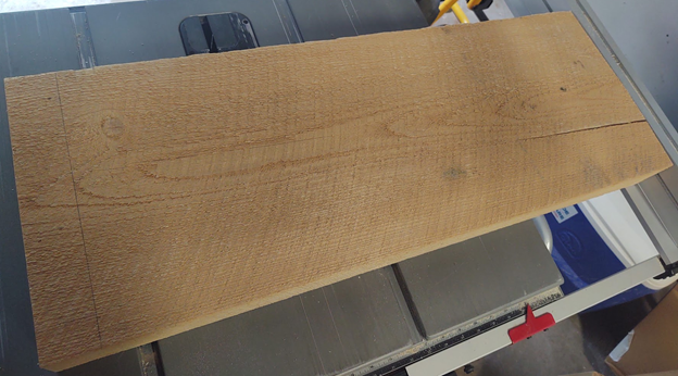
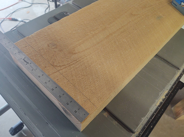
One of my favorite activities is wood working. I am not particularly skilled in the art, but I enjoy using the tools, building useful things, and admiring the beauty of the natural product. I often tell people that “getting good” at wood working is all about learning how to measure, gauge and build the fixtures to carry out an operation. When you have a chunk of wood, one of the most fundamental operations is to measure its length against some fixed standard. Let us begin with a beautiful chunk of Eastern Hemlock:
Figure 2. A 12” x 3” x 26” Piece of rough sawn eastern hemlock.
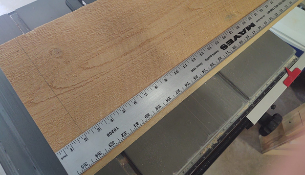
One of the first things we might want to do to with this specimen is use some sort of standard gauge to compare it to:
Figure 3. Comparing our wood against a reference.
We can pick a standard unit and compare our specimen to a scale based upon that unit. In my case the unit was “inches” of length, but it could be anything that helps up solve our problem at hand. Often you want to pick a unit and coordinate system that scales well to the problem at hand. If we want to measure circular “things”, we might use a protractor as it makes understanding the measurement easier. The idea is to work in a system that is in the “coordinate system” of your problem. It makes sense to use a ruler to measure a “rectangular” piece of wood.
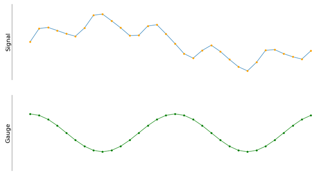
What does this have to do with DSP and Fourier transforms? I hope to show you that a Fourier Transform (and its efficient discrete implementation, the FFT) is a set of gauges that can be used to understand a time domain signal. We can use the PowerQuad hardware to carryout out the “gauging”. For the sake of this discussion, let us consider a time domain signal such as this:
Figure 4. An example time-domain signal
This particular signal is a bit more complex than the simple sine wave used in previous articles. How exactly would we “gauge” this signal? Amplitude? Frequency? Compute statistics such as variance? Most real-world signals can have quite a bit of complexity, especially when they are tied to some physical process. For example, if we are a looking at the result of some sort of vibration measurement, the signal could look very complicated as there are many physical processes contributing to the shape. In vibration analysis, the physical “things” we are examining with move and vibrate according to well understood physics. The physics show that the systems can be modeled with even order differential equations. This means always be we can write the behavior of the system over time as the sum of sinusoidal oscillations. So, what would be a good gauge to use to examine our signal? Well, we could start with a cosine wave at some frequency of interest:
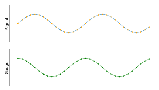
Figure 5. Gauging our signal against a cosine wave.
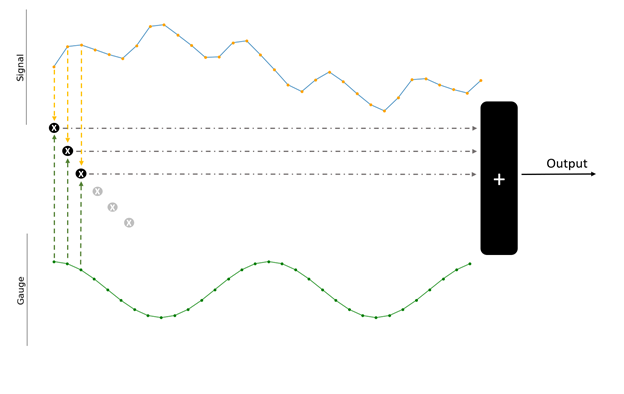
Choosing a cosine signal as a reference gauge can simplify the problem as we can easily identify the properties of our unit of measure, i.e. its frequency and amplitude. We can fix the amplitude and frequency of our reference and then compare it to our signal. If we do our math correctly, we can get a number that indicates how well correlated our input signal is to a cosine wave of a particular frequency and a unit amplitude. So, how exactly do we perform this correlation? It turns out to be a simple operation. If we think about the input signal and our reference gauge as discrete arrays of numbers (i.e. vectors), we can compute the dot-product between them:
Figure 6. Computing the correlation between a test signal and our feference gauge.
The operation is straightforward. Both your signal input and the “gauge” has the same number of samples. Multiply the elements of each array together and add up the results. Using an array like notation, the input is represented by “x[n]” and the gauge is represented by “re[n]” where n is an index in the array:
Output = x[0]*re[0] + x[1]*re[1] + x [2]*re[2] + . . .
What we end up with is a single number (scalar). Its magnitude is proportional to how well correlated out signal is to the particular gauge we are using. As a test, you could write some code and use a cosine wave as your input signal. The test code could adjust the frequency of input and as the frequency of the input gets closer to the frequency of the gauge, the magnitude of the output would go up.
As you can see the math here is just a bunch of multiplies and adds, just like the IIR filter from our last article. There is one flaw however with this approach. There is special case of the input where the output will be zero. If the signal input is a cosine wave of the *exact* frequency as the gauge and is 90 degrees phase shifted with respect to the reference gauge, we would get a zero output.
Figure 7. A special case of our reference gauge that would render zero output.
This is not desirable as we can see that input is correlated our reference gauge, it just is shifted a in time. There is a simple fix and we can even use our piece of hemlock lumber to illustrate.
Figure 8. Gauging along a different side of the lumber.
In Figure 3, I showed a ruler along the longest length of the wood. We can also rotate the ruler and measure along the shorter side. It is the same gauge, just used a different way. Imagine that board was only 1” wide but 24” long. I could ask an assistant to use a ruler and measure the board. Which of those two numbers is “correct”? The assistant could report to me either of those numbers and be technically correct. We humans generally assume length to be the longer side of a rectangular object but there is nothing special about that convention. In figure 6, we were only measuring along 1 “side” of the signal. It is possible to get a measurement that is zero (or very small) while have a signal that looks very similar to the gauge (like in figure 7). We can fix this by “rotating” our ruler similar to figure 8 and measure along the both ”sides” of the signal.
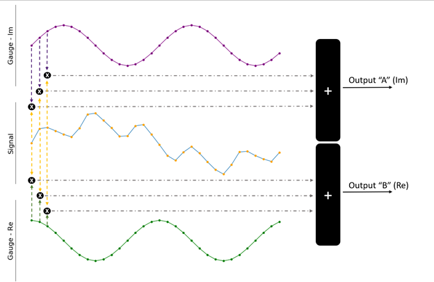
Figure 9. Using two reference gauges. One is “rotated” 90 degrees.
In figure 9, I added another “gauge” labeled “A” in purple. The original gauge is labeled “B”. The only difference between the two gauges is that B is phase shifted by 90 degrees. This is equivalent to rotating my ruler in figure 8 and measuring the “width” of my board. In figure 9, I am showing 3 of the necessary multiply/add operations but you would carry out the multiple/add for all points in the signal. Writing it out:
B = x[0]*Re[0] + x[1]*Re[1] + x [2]*Re[2] + . . .
A = x[0]*Im[0] + x[1]*Im[1] + x [2]*Im[2] + . . .
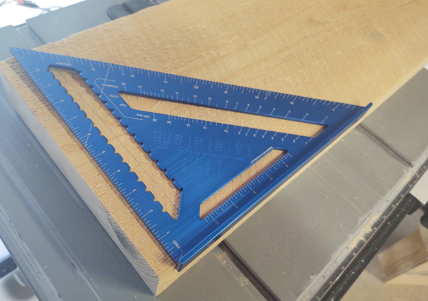
In this new formulation we get a pair of numbers A,B for our output. Keep in mind that we are gauging our input against a *single* frequency of reference signals at a unit amplitude. This is analogous to measuring the length and width of our block of wood. Another way of thinking about it is that we now have a measuring tool that evaluates along 2 axes which are “orthogonal”. It is almost like a triangle square.
Figure 10. A two-axis gauge.
Once we have our values A & B, it is typical to consider them as a single complex number
Output = B + iA
The complex output gives us a relative measure of how we are correlated to our reference gauges. To get a relative amplitude, simply compute the magnitude:
||Output|| = sqrt(A^2 + B^2)
You could even extract the phase:
Phase = arctan(B/A)
It common to think about the output in “polar” form (magnitude/phase). In vibration applications you typical want understand the magnitude of the energy at different frequency components of a signal. There are applications in communications, such as orthogonal frequency domain multiplexing (OFDM), where you work directly the with real and imaginary components.
I previously stated that the correlation we were performing is essentially a vector dot product operation. The dot product shows up in many applications. One of which is dealing with vectors of length 2 where we use the following relationship:
The interesting point here is that the dot product is a simple way of getting a relationship of the angle and magnitude between two vectors and b. It is easy to think about a and b as vectors on a 2d plane, but the relationship extends to vectors of any length. For digital data, we work with discrete samples, so we define everything in terms of the dot product. We are effectively using this operation to compute magnitudes and find angles between “signals”. In the continuous time world, there is the concept of the inner-product space. It is the “analog” equivalent of the dot product that underpins the mathematical models for many physical systems.
At this point we could stop and have a brute force technique of comparing a signal against a single frequency reference. If we want to determine if a signal had a large component of a particular frequency, we could tailor our reference gauges to the *exact* frequency we are looking for. The next logical step is to compare our signal against a *range* of reference gauges of different frequencies:
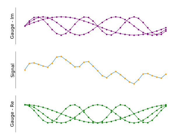
Figure 11: Using a range of reference gauges at different frequencies.
In Figure 11, I show four different reference gauges at frequencies that have an integer multiple relationship. There is no limit to the number of frequencies you could use. With this technique, we can now generate a “spectrum” of outputs at all the frequencies of interest for a problem. This operation has a name: the Discrete Fourier Transform (DFT). One way of writing the operation is:
Figure 12. The Discrete Fourier Transform (DFT)
N is the number of samples in the input signal.
k is the frequency of the cosine/sine reference gauges. We can generate a “frequency” spectrum by computing DFT over a range of “k” values. It is common to use a linear spacing in when selecting the frequencies. For example, if your sample rate is 48KHz and you are using N=64 samples, it is common (we will see why later) to use 64 reference gauges spaced at (48000/64)Hz apart.
The “Fast Fourier Transform”
The Fast Fourier Transform is a numerically efficient method of computing the DFT. It was developed by J. W. Cooley and John Tukey in 1965 as a method of performing the computation with a fewer adds and multiplies as compared to the direct implementation shown in Figure 11. The development of the FFT was significant as we can do our number crunching much more efficiently by imposing a few restrictions on the input. There are a few practical constraints that need to be considered when using an FFT implementation
- The length of your input must be a power of 2. i.e. 32, 64, 128, 256.
- The “bins” of the output are spaced in frequency by the sample rate of your signal divided by the number of samples in the input. As an example, if you have a 256-point signal sampled at 48Khz, the array of outputs corresponds to frequencies spaced at 187Hz. In this case the “bins” would correlate to 0Hz, 187.5Hz, 375 Hz, etc. You cannot have arbitrary input lengths or arbitrary frequency spacing in the output.
- When the input the FFT/DFT are “real numbers” (i.e. samples from an ADC), the array of results exhibits a special symmetry. Consider an input array of 256 samples. The FFT result will be 256 complex numbers. The 2nd half of the output are a “mirror” (complex conjugates) of the 1st half. This means that for a 256-sample input, you get 128 usable “bins” of information. Each bin has a real and imaginary component. Using our example in #2, the bins would be aligned to 0Hz, 187.5Hz, 375Hz, all the way up to one half of our sample rate (24KHz).
You can read more details about how the FFT works as well as find plenty of instructional videos on the web. Fundamentally, the algorithm expresses the DFT of signal length N recursively in terms of two DFTs of size N/2. This process is repeated until you cannot divide the intermediate results any further. This means you must start with a power of 2 length. This particular formulation is called the Radix-2 Decimation in Time (DIT) Fast Fourier Transform. The algorithm gains its speed by re-using the results of intermediate computations to compute multiple DFT outputs. The PowerQuad uses a formulation called “Radix-8” but the same principles apply.
Using the PowerQuad FFT Engine
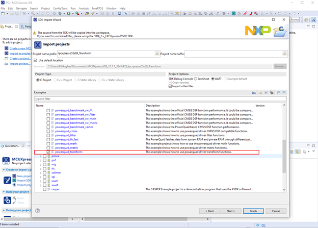
The underlying math to a DFT/FFT boils down to multiplies and adds along with some buffer management. The implementation can be pure software, but this algorithm is a perfect use case for a dedicated coprocessor. The good news is that once you understand the inputs and outputs of a DFT/FFT, using the PowerQuad is quite simple and you can really accelerate your particular processing task. The best way to get started with using the PowerQuad FFT is to look at the examples in the SDK. There is an example project called “powerquad_transform” which has examples that test the PowerQuad hardware.
Figure 13. PowerQuad Transform examples in the MCUXpresso SDK for the LPC55S69
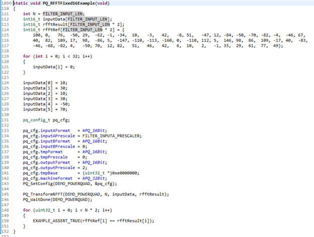
In the file powerquad_transform.c, there are several functions that will test the PowerQuad engine in its different modes. For now, we are going to focus on the function PQ_RFFTFixed16Example(void).
This example will set up the PowerQuad to accept data in a 16-bit fixed point format. To test the PowerQuad, a known sequence of input and output data is used to verify results. The first thing I would like to point out is that the PowerQuad transform engine is used fixed point/integer processing only. If you need floating point, you will need to convert beforehand. This is possible with the matrix engine in the PowerQuad. I personally only every use FFTs with fixed point data most of my source data comes right from analog to digital converter data. Because of the processing gain of the FFT, I have never seen any benefit of using a floating-point format for FFTs other than some ease of use for the programmer. Let us look at the buffers used in the example:
Notice that the input data length FILTER_INPUT_LEN (which is 32 samples). The arrays used to store the outputs are twice the length. Remember that an FFT will produce the same number of *complex* samples in the output as there are samples for the input. Since our input sample are real values (scalars) and the outputs have real/imaginary components, it follows that we 2x the length to storage the result. I stated before that one of implications of the FFT with real valued inputs is that we have a mirror spectrum with complex conjugate pairs. Focusing on the reference for testing the FFT output in the code:
The 1st pair 100,0 corresponds to the 1st bin which is a “DC” or 0Hz component. It should always have a “zero” for the imaginary component. The next bins can be paired up with bins from the opposite end of the data:
76,-50 <-> 77,49
29,-62 <-> 29, 61
-1, -34 <-> -1,33
These are the complex conjugate pairs exhibiting mirror symmetry. You can see that they are not quite equal. We will see why in a moment. After all the test data in initialized, there is a data structure used to initialize the PowerQuad:
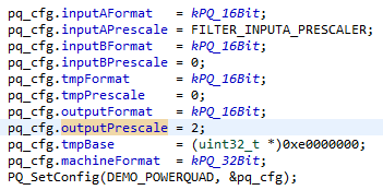
One of the side effects of computing an FFT is that you get gain at every stage of the process. When using integers, it is possible to get clipping/saturation and the input needs to be downscaled to ensure the signal down not numerically overflow during the FFT process. The macro FILTER_INPUTA_PRESCALER is set to “5”. This comes from the length of the input being 32 samples or 2^5. The core function of the Radix-2 FFT is to keep splitting the input signal in half until you get to a 2-point DFT. It follows that we need to downscale by 2^5 as we can possible double the intermediate results at each stage in the FFT. The PowerQuad uses a Radix-8 algorithm, but the need for downscaling is effectively the same. I believe that some of the inaccuracy we saw in the complex conjugates pairs the test data was from the combination of an input array values that are numerical small and the pre-scale setting. Note that the pre-scaling is a built in hardware function of the PowerQuad.
The PowerQuad needs an intermediate area to work from. There is a special 16KB region starting at address 0xe0000000 dedicated to the PowerQuad. The PowerQuad has a 128-bit interface to this region so it is optimal to use this region for the FFT temporary working area. You can find more details about this private RAM in AN12292 and AN12383.
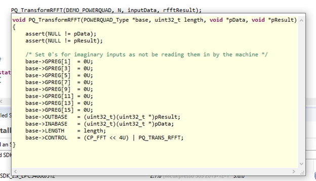
Once you configure the PowerQuad, the next step is to tell the PowerQuad the input and result data is stored with the function PQ_transformRFFT().
Notice in the implementation of the function, all that is happening is setting some more configuration registers over the AHB bus and kicking off the PowerQuad with a write to the CONTROL register. In the example code, the CPU blocks until the PowerQuad is finished and then checks the results. It is important to point out that in your own application, you do not have to block until the PowerQuad is finished. You could setup an interrupt handler to flag completion and do other work with the general purpose M33 core. Like I stated in my article on IIR filtering with the PowerQuad, the example code is a good place to start but there are many opportunities to optimize your particular algorithm. Example code tends to include additional logic to check function arguments to make the initial experience better. Always take the time look through the code to see where you can remove boilerplate that might not be useful.
Parting Thoughts
- The PowerQuad includes a special engine for computing Fast Fourier Transforms.
- The FFT is an efficient implementations of the Discrete Fourier Transform. This process just compares a signal against a known set of reference gauges (Sines and Cosines)
- The PowerQuad has a private region to do its intermediate work. Use it for best throughput.
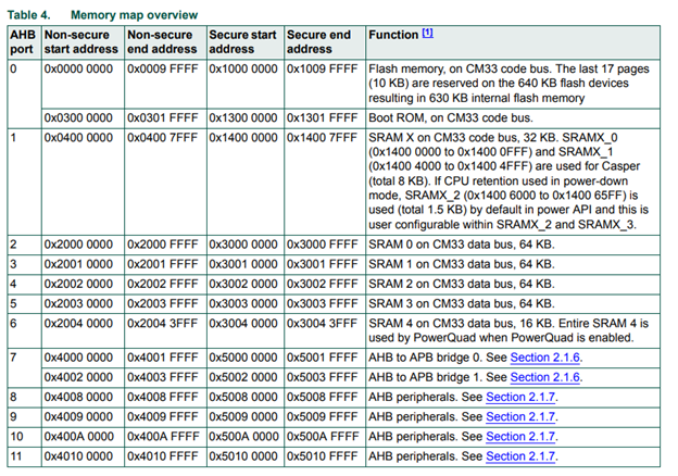
- Also consider the memory layout and AHB connections of where your input and output data lives. There may be additional performance gains by making sure you input DSP data is in a RAM block that is on a different port than RAM used in your application for general purpose task. This can help with contention when different processes are accessing data. For example, SRAM0–3 are all on different AHB ports. You might consider locating you input/output data in SRAM3 and having your general-purpose data in SRAM0-2. Note: You still need to use 0xE0000000 for the PowerQuad TEMP configuration for its intermediate working area.
At this point you can begin looking through the example transform code. Also make sure to read through AN12292 and AN12383 for more details. While there are more nuances and details to FFT and “frequency domain” processing, I will save those for future articles. Next time I hope to show some demos of the PowerQuad FFT performance on the Mini-Monkey and illustrate some other aspect of the PowerQuad. Until then, check out some of the additional resources below on the LPC55S69.
Additional LPC55S69 resources:
https://community.nxp.com/videos/9003
https://community.nxp.com/videos/8998
You must be a registered user to add a comment. If you've already registered, sign in. Otherwise, register and sign in.
-
101
6 -
communication standards
4 -
General Purpose Microcontrollers
19 -
i.MX RT Processors
45 -
i.MX Processors
43 -
introduction
9 -
LPC Microcontrollers
73 -
MCUXpresso
32 -
MCUXpresso Secure Provisioning Tool
1 -
MCUXpresso Conig Tools
30 -
MCUXpresso IDE
40 -
MCUXpresso SDK
25 -
Model-Based Design Toolbox
6 -
MQX Software Solutions
2 -
QorIQ Processing Platforms
1 -
QorIQ Devices
5 -
S32N Processors
4 -
S32Z|E Processors
6 -
SW | Downloads
4
- « Previous
- Next »

