- NXP Forums
- Product Forums
- General Purpose MicrocontrollersGeneral Purpose Microcontrollers
- i.MX Forumsi.MX Forums
- QorIQ Processing PlatformsQorIQ Processing Platforms
- Identification and SecurityIdentification and Security
- Power ManagementPower Management
- MCX Microcontrollers
- S32G
- S32K
- S32V
- MPC5xxx
- Other NXP Products
- Wireless Connectivity
- S12 / MagniV Microcontrollers
- Powertrain and Electrification Analog Drivers
- Sensors
- Vybrid Processors
- Digital Signal Controllers
- 8-bit Microcontrollers
- ColdFire/68K Microcontrollers and Processors
- PowerQUICC Processors
- OSBDM and TBDML
-
- Solution Forums
- Software Forums
- MCUXpresso Software and ToolsMCUXpresso Software and Tools
- CodeWarriorCodeWarrior
- MQX Software SolutionsMQX Software Solutions
- Model-Based Design Toolbox (MBDT)Model-Based Design Toolbox (MBDT)
- FreeMASTER
- eIQ Machine Learning Software
- Embedded Software and Tools Clinic
- S32 SDK
- S32 Design Studio
- Vigiles
- GUI Guider
- Zephyr Project
- Voice Technology
- Application Software Packs
- Secure Provisioning SDK (SPSDK)
- Processor Expert Software
-
- Topics
- Mobile Robotics - Drones and RoversMobile Robotics - Drones and Rovers
- NXP Training ContentNXP Training Content
- University ProgramsUniversity Programs
- Rapid IoT
- NXP Designs
- SafeAssure-Community
- OSS Security & Maintenance
- Using Our Community
-
-
- Home
- :
- モデルベース・デザイン・ツールボックス(MBDT)
- :
- NXPモデルベース・デザイン・ツールナレッジベース
- :
- Classical and Modern Algorithms for Trajectory and Speed Control of an Autonomous Vechicle
Classical and Modern Algorithms for Trajectory and Speed Control of an Autonomous Vechicle
- RSS フィードを購読する
- 新着としてマーク
- 既読としてマーク
- ブックマーク
- 購読
- 印刷用ページ
- 不適切なコンテンツを報告
Classical and Modern Algorithms for Trajectory and Speed Control of an Autonomous Vechicle
Classical and Modern Algorithms for Trajectory and Speed Control of an Autonomous Vechicle
1. Introduction
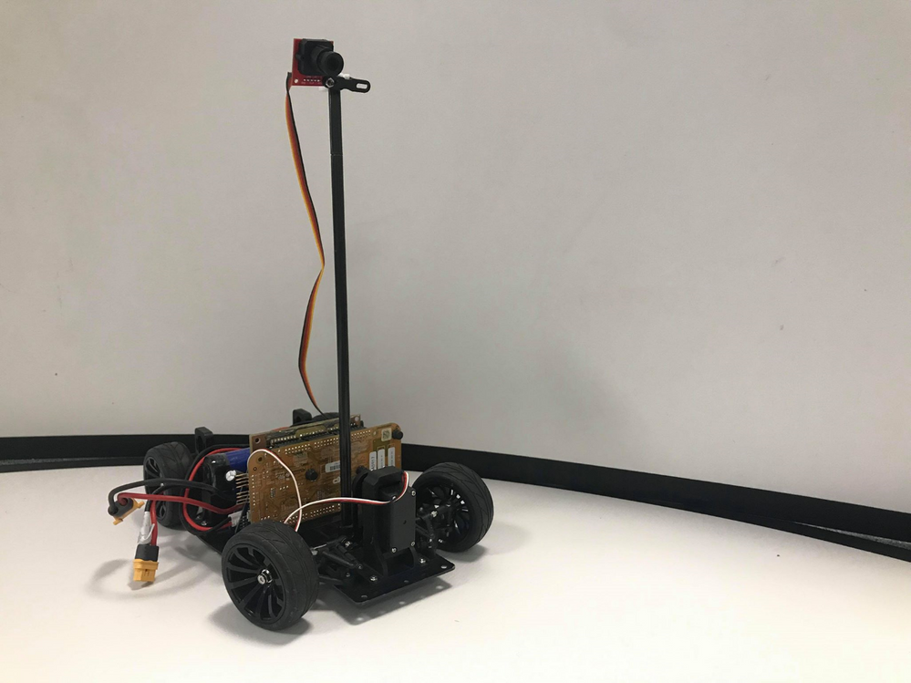
This article discusses various algorithms for controlling trajectory and speed for an autonomous vehicle. The car is built with S32K144 and the NXP's Cup car chassis as explained in depth in this article: https://community.nxp.com/docs/DOC-341984. All software used for programming the car is done using MATLAB/Simulink toolbox called Model-Based Design Toolbox for S32K1xx - NXP Support Package S32K1xx - File Exchange - MATLAB Central. The goal of achieving imposed performances for this system is approached in a classical manner using a PID (Proportional Integral Derivative) controller and also by using modern control algorithms: LQG (Linear Quadratic Gaussian), LTR (Loop Transfer Recovery), H2 and H∞.
2. Vehicle Dynamics Model
A logical way of creating a formal representation of the physical system is described in the following section. The significant contribution of such representation is outlined in the control algorithms design process. Validation of these algorithms in a simulation environment, where a mathematical model approximates the real system, is a procedure which is going to be undertaken to ensure rectitude and precision for the developed solutions. Simplifying assumptions must be made to create the context of ease in manipulating such a formal representation, considering the existing numerical algorithms. Therefore, the mathematical model will possesses a certain level of compromise between the simplicity of the representation and accuracy related to the real system.
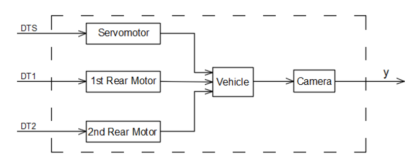
Before starting to model the car’s dynamics, a brief analysis of the system is introduced to offer a clear image on the process. The car can be controlled through three independent inputs, duty cycles which are given as inputs to the Simulink blocks: the duty cycle for the servomotor; the duty cycle for the 1st rear wheel and the duty cycle for the 2nd rear wheel. The output of the process is represented by the image camera sees in front of it, the array Y with the converted values of the analog signal transmitted by the sensor. Hence, a Multiple Input Single Output (MISO) process is modeled in the current section of the paper. The actuators are represented by the three motors, two to ensure traction of the car, and one servomotor responsible for the steering. The plant is represented by the actual vehicle, and the sensor is constituted by the camera which provides the image in front of the car. Thereby, Figure 2.1 illustrates the correspondence between the physical ensemble and the control theory components.
Figure 2.1 Actuators, plant, sensor
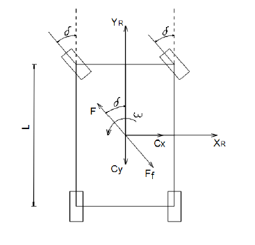
Before exposing the equations that describe the dynamics of the system, a representation of the forces that affect the vehicle is illustrated in Figure 2.2, where: XR and YR define the robot frame, δ represents the turning angle of the front wheels, F is the traction force generated by the two DC motors of the rear wheels, Ff denotes the friction force that the vehicle must overcome during its movement, L is the length of the car, measured from the center of the front wheels to the center of the rear wheels, Cx and Cy reactive forces depending on the movement velocity and ω the angular velocity.
Figure 2.2 Forces acting on the vehicle
Now, writing Newton’s law for the translation motion and considering the decomposition of the forces on the robot’s frame axis, the motion is described as well as longitudinal as latitudinal by:
The traction and resistance forces can be expressed based on the two DC motors parameters:
where: ui - voltage applied on the inner wheel motor, uo - voltage applied on the outer wheel motor (related to turning behavior), km - DC motor constant, rw - rear wheels diameter, R - winding resistance, Bv - resistance coefficient for the translation motion, μ - friction coefficient, M - mass of the vehicle, g - gravitational acceleration. When it comes to the rotational motion, the equation which describes the vehicle dynamics is given by:
where: MFx - moment of Fx force, Md - moment caused by the difference of speeds on the two rear wheels which triggers the car to change its orientation, MFfx - moment of Ffx force, which opposes to the rotational movement, Cw - reaction dependent to the angular velocity and J - moment of inertia.
Considering thus the previous formulas for the traction and friction force, the final equation of the rotational movement is:
where all the variables have the same meanings as already specified and more than that, Bw represents the resistance coefficient for the rotational motion.
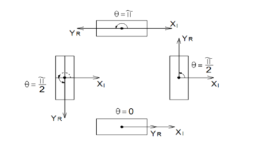
To express the position of the vehicle on the track, an approach based on angles is going to be used to provide a suitable functional description of the process. Therefore, θ represents the angle between the YR-axis of the robot and the XI-axis of an inertial frame, like in Figure 2.3 The θ angle provides information about the car’s position on the given track, and it represents the variable to be measured to ensure the desired behavior of the vehicle.
Figure 2.3 System output - θ angle
Therefore, the differential equations that model the vehicle’s dynamics are written in the inertial coordinate system and obtained considering a Newtonian approach as in:
The mathematical representation given by the previous differential equations is characterized by nonlinear dynamics. A linearization procedure is therefore implemented to obtain a state-space representation of the given model. For the particular model developed so far, considering the variables and their signification related to the vehicle’s dynamics, the state array is formed by: x' = [θ vx vy ω], while θ represents the output and u' = [δ ui uo] defines the control signals array.
The differential equations of the vehicle dynamics are introduced in the Simulink environment for obtaining the linear system. Input and output ports are used for the controlled and measured variables, while a simple logic of mathematical operations blocks, integrator blocks, and signals connections are implemented. Before using the linmod Matlab function to obtain the linearized model, a static operating point must be chosen. When it comes to this, the following assumptions are made: the car travels a straight road, the front wheels are straight, no turning angle, the rear wheels have equal rotational speed and the car is perpendicular on the X-axis of the inertial system coordinate. All these specifications correspond to a duty cycle equal to 0.03, as mentioned previously. For the two rear wheels, a 10% speed is chosen. However, the transfer from the duty cycles transmitted to the motors and the inputs considered for the system in the current model should also be computed.
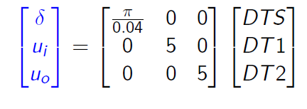
For the two rear DC motors, the voltage applied is proportional to the duty cycle control signal. A 0% duty cycle (no rotational speed) is equal to a 0V power voltage. While the maximum voltage of the DC motors is 5V, and the maximum duty cycle is 100%, it is easy to determine the proportionality factor, which is equal to 5. When it comes to the conversion between the duty cycle of the servomotor and the turning angle of the front wheels, it must be taken into account that the maximum angle physically achievable for the front wheels is equal to 45 degrees. Therefore, the transfer can be modeled by:
With all the transfers modeled and all the model's constants replaced with numerical values, a state-space representation is computed for the entire process and the system is described by the following minimal state-space representation:
3. Control Algorithms
3.1 Experimental PID Position Control
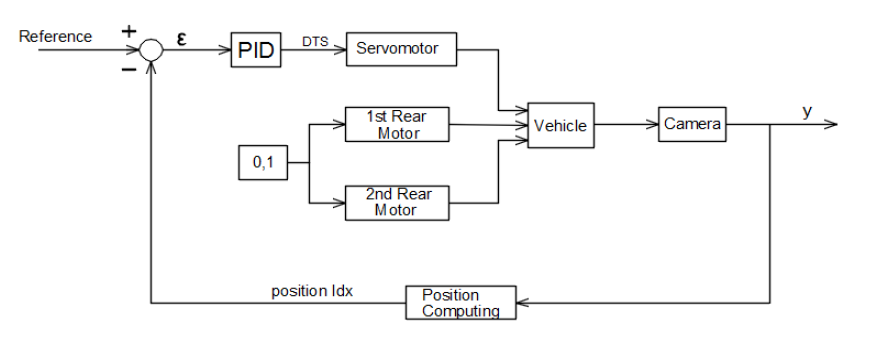
The actual position of the car on the track is compared to a defined reference and it is desired to maintain the error between these variables as small as possible, with the purpose mentioned in the previous paragraph. The inputs on the rear motors are given by a constant duty cycle equal to 0.1, which represents 10% of the maximum speed that the car can reach. All these information are represented in a schematic manner in Figure 3.1.1
Figure 3.1.1 Position control loop
3.1.1 Position Computing and Reference Defining
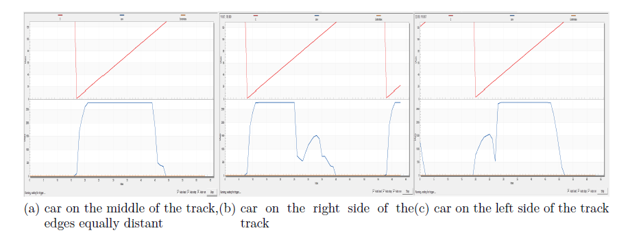
Relying on the array of intensities returned by the ADC, the following procedure was undertaken to gain knowledge about what the camera sees. The robot was firstly placed on one side of the track, and connected to the FreeMaster tool for real-time data collecting. The experiment was repeated for different positions of the vehicle, and the results are illustrated in the figures below:
Figure 3.1.1.1 Exemplification of what camera sees for different positions of the car on the track
Noticing how the image in front of the camera changes related to its position, it is desirable for the two dips on the graphics to be equally distant from the center of the array. A position finding algorithm is therefore implemented for searching the edges of the road.
3.1.2 Parameters Tunning
Based on the error value, the steering input is computed. Bearing in mind the fact that the duty cycle for the servomotor should be in the range of 0.02 – 0.04, the control signal given to the actuator should be bounded for this particular input range. Thus, a scaling factor is introduced before the error is transmitted to the controller. Considering the error range, a convenient scaling factor is chosen.
Irrespective of the correspondence of the errors to left or right halves of the road displacements, the magnitude of the signal should be processed by the controller in the same way. The symmetry has then to be dismissed because different values of the duty cycle should be computed to make the car turn left or right. Therefore, the PID controller can return a control signal which is maximum equal to 0.01, for an maximum error value, which then, based on the sign of the position index algorithm returned value, should be added to 0.03 (wheels not steered) for a movement to the left, or subtracted from 0.03 for a movement to the right.
Following all the introduced information, the first step into the procedure of tuning the PID controller is to build a proportional controller. A maximum error value, divided by the scaling factor corresponds to a maximum 0.01 control signal. Moreover, knowing that for a proportional controller, which is discrete considering its use directly on the real process:
the proportional parameter of the PID controller is computed from the previous formula.
The result of the designed controlled system is now illustrated in Figure 3.1.2.1, extracted from the FreeMaster debug tool in real time, while the car completes multiple laps on the given track.The output of the system is illustrated on the Y-axis, the reference is marked with a black line, and the time scale is represented on the X-axis, in seconds. The dips on the graphical representation of the system’s output correspond to the curvatures of the road, where a significant error triggers the wheels steering to keep the car on the track. The wavy portion is the system’s output on the wavy piece of the road, and the almost straight area is the output provided when the car is on the straight piece of the track. It is noticeable that on the straight part of the track, the reference is not completely followed. Also, on a long straight road, only the proportional component is not able to ensure a steady state error equal to zero.
Figure 3.1.2.1 System reference and output with P controller
Figure 3.1.2.2 Track components: straight, curve, wavy
Rising even more the KR factor value does not solve this problem, because the risk of the system’s instability appears in this scenario. Thus, the integrative component should be used, and now the controller is a PI, with the following control law:
The Ti value is chosen experimentally, and satisfying results are illustrated in the following figure:
Figure 3.1.2.3 System reference and output with PI controller
A derivative component is not necessarily required, considering the form of the track (without sudden changes of direction). Inside the PID block which implements the controller in the Simulink environment, besides the parameters choice and also the upper and lower saturation limits of the control signal, the clamping anti-windup method is also used for preventing the controller output from saturating. The sampling time is left to be inherited, this option allowing the Matlab environment to choose the right sampling period considered regarding the timing in the given Simulink model.
3.2 Experimental PID Speed Control
The center of the track is now followed, and the behavior of the vehicle is as desired. On longer tracks, the vehicle movement seems like a crawl, and the particularities of the system allow the control of three different inputs. A speed control algorithm is thus implemented to ensure a reduced time in completing a lap.
Like any other car, the robot should be able to adapt its speed depending on the track to be traversed. Acceleration and deceleration features should be implemented into the current application to emulate the behavior of a real-life vehicle. Also depending on the road’s particularities, curvatures, distances, a speed limit should be left to be user’s choice.
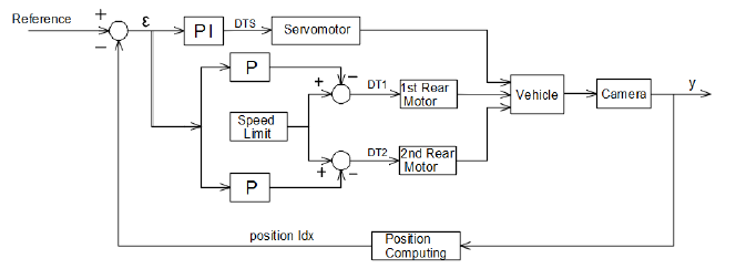
Intuitively, from a driver perspective, the speed should be reduced at the beginning of the curve and then gradually increased on the second part of the curve, as the car leaves it and heads to a straight piece of the road. Taking into consideration this real life behavior, the graphic evolution of the output of the system controlled with the PID position controller seems to illustrate this exact idea. It is noticeable that inside a curve, the error slowly increases as the car approaches the center of the turn, and then decreases while the exit becomes close. A proportional control signal to the speed of the two wheels can be thus computed to take care of this operating mode.The error signal is consequently fed to a P controller which amplifies it considering, for the beginning, that the maximum speed allowed is equal to 0.15 (15%). Therefore, the control loop is completed, as illustrated in the figure below:
Figure 3.2.1 Position and speed control loop
Assuming that the imposed speed limit is provided by a duty cycle equal to 0.15, as specified in the previous paragraph, and also that, during a turn, it must be reduced to 0.1, the KR factor of the two controllers, one for each rear wheel is given by:
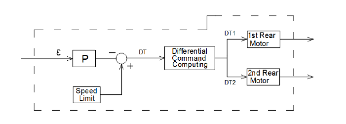
The KR general formula can be modified under the desired speed range (how fast should the car go and how fast should it take turns). The control signal given to the rear motors, uk = KRϵk is subtracted from the imposed speed limit to achieve the desired behavior on the curvatures of the road. The car travels the track faster now, but increasing the speed, even more, causes a side-slip of the vehicle during turns. This shortcoming could be improved by taking advantage of the fact that the two rear wheels can be controlled independently. Hence, inside a turn, the outer wheel should have a bigger rotation speed than the inner one, in the same way, an automobile operates. This differential control of the traction wheels is used to increase the stability of the system, improving, therefore, the performances of the vehicle.
However, a way of computing the difference between the speeds of the two rear wheels must be implemented. The overall speed of the moving vehicle is given by the two duty cycle control signals, and it is:
The ratio between the outer wheel speed and the inner wheel speed is experimentally chosen based on the formula:
The experimental procedure is undertaken for obtaining a suitable value for the speed ratio started by choosing this factor equal to 1. For a speed ratio equal to 1 there is no differential control of the rear wheels, both of them having the same rotation speed. The speed ratio produced satisfactory results for a value equal to 1.3. A 1.4-speed ratio factor is also suitable for the application, but increasing it more could cause unwanted behaviors such as the car turning around its axis.
With a 1.3-speed ratio factor, a 20% (0.2) speed limit was achieved, with a lower value of 15% (0.15) during turns. Increasing the speed, even more, 25% (0.25) and keeping the lower value at its previous setting produces, in some cases, side-slips of the vehicle outside the track. By reducing the vehicle turning speed, for example, 10% (0.1) does not solve the side-slip issue. The leading cause of this behavior is related to the oval shape of the track, with short straight segments. As on a winding road, the robot should also limit its speed because sudden acceleration and deceleration actions cause undesired system’s reactions and safety issues are definitely to be considered during control algorithms design. Mixing this way of computing two different duty cycles for the two rear wheels, with the proportional controller introduced in the first part of this subsection, which will provide the overall DT, the vehicle shows more stability during the turns than it did without the differential speed control and a bigger speed can be achieved without losing the position requirements.
Figure 3.2.2 Computing the rear wheels control signals
3.3 LQG and LTR
Unlike the PID regulator, the LQG and LTR control laws are going to be designed in a theoretical manner, based on the mathematical model of the system, obtained in the previous section. However, before implementing the controllers in the Simulink environment for proper simulation and validation of their results, a short analysis of the open loop system is going to be depicted in the next subsection.
3.3.1 Position Computing and Reference Defining
As illustrated in the previous chapter of the thesis, the output of the mathematical representation is the angle θ measured between the Y-axis of the robot frame and the X-axis coordinate of the inertial frame. There are also three inputs of the system given by the values of the duty cycles transmitted to the motors.
Thereby, the four matrices,A,B,C and D are introduced as a state-space block in a newly created model in the Simulink environment.
However, the simulation does not recognize the output of the system as an angle. Considering the work in a digital environment, its values are increasing and decreasing following the given inputs. This behavior is as expected, assuming that a constant speed on the rear wheels and a certain angle of the front ones produces a variation of the output, increasing or decreasing its value based on the steering direction. However, the output θ is an angle, so the subsequent processing of the signal is realized. The following assumptions are made: the value of θ is measured trigonometrical; the minimum value for θ is 0 radians, and the maximum value for θ is π.
It is natural that for bigger angles than π, the real value of the angle is computed by theta real = theta measured − π. Before applying this verification and then modification of the measured value, it must be made sure that the output of the system is not negative; therefore a Simulink block is used to compute its absolute value.
Figure 3.3.1.1 Theta angle conversion
As noticeable in the previous figure, the system’s output changes its value when the vehicle is going inside curvature of the road, for example. As assumed during the linearization procedure, the car starts its movement from a position which is perpendicular on the X-axis of the inertial coordinate system, thus leading to a θ equal to π/2 .
If the camera spots a dark value in front of the car, which represents a black edge that needs to not be crossed, based on the position where the edge is seen, a deviation angle α will be computed in order to express the fact that the car needs to change its direction, less or more abruptly.
Based on this deviation angle, the reference of the control loop is going to change its value to determine the vehicle to turn when edges are spotted. Therefore the reference of the system will be given by: θ+α, with θ the system’s output. From the way of measuring the α angle, given by the following figure, it can be concluded that a positive α angle determines to steer to the left, while a negative one determines the steering to the right, as explicitly illustrated in the following figure:
Figure 3.3.1.2 Deviations regarding the trajectory to be followed
3.3.2 Controller Implementation
Firtsly, an LQG controller is implemented in the Simulink environment using the lqg Matlab function:
where sys is the state-space representation of the system given by the A,B,C and D matrices. QXU is the penalty matrix considering that the cost function to be minimized by the algorithm is written as:
The QWU noise covariance matrix is given by:
The control signal u is computed with the help of an LQR (Linear Quadratic Regulator) such that J reaches is minimum value. A Riccati equation depending on the state-space representation of the system and the penalty matrices Q and R is solved with this purpose, but these details are not subject of the current description. However, for obtaining such a controller, a full state array x is required. The feasibility of this assumption is not guaranteed considering that in many control problems, not all the state components are measurable. If moreover, the process is affected by noise, a Kalman filter has to be used. After the Kalman filter estimates the full state of the system, the LQR algorithm computes optimally the control signal, based on the state estimation. This procedure is called the synthesis of a LQG controller.
Considering the penalty of the state deviation which needs to be accomplished and also the control signals limitations required for a safety operation mode, the values of these matrices are chosen conveniently. The returned controller is given by a state-space representation which is introduced into a state-space block in Simulink, and connected to the system considering a classical control loop. However, before doing so, the obtained controller is sampled with a convenient sampling period to ensure the functionality of the given process, using the c2d Matlab command.
The control signals given by the discrete controller, before being fed to the system, are added to their linearization values and saturation blocks are also used to prevent the damages a very high control signal can produce on the system’s actuators. The implementation on the real system is illustrated in the figure below, where the deviation based on the array returned from the camera is given to the controller as an error signal, as mentioned previously.
Figure 3.3.2.1 LQG control loop on the real system
As mentioned previously, LQG controller is formed by a LQR and a Kalman filter. However, when using a Kalman estimator together with a linear quadratic regulator, the robustness of the designed algorithm deteriorates. To overcome this loss of robustness, the LTR methodology is used in this example, as a second control option, to recover the robustness of the linear-quadratic regulator through a modified computation of this controller.
The same reference defining and position computing apply also for the LTR algorithm as well. No modifications are brought to the control loop, except for the controller, which is now computed using the ltrsyn command:
where sys is the state-space representation given by the A,B,C and D matrices in. Kf represents the optimal gain filter matrix, while Qf and Rf are identity noise covariance matrices. The recovery of the full-state feedback linear quadratic loop is thus realized with a gain specified by RHO.
3.4 H2 and H∞
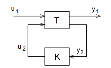
Considering the particularities of the current application, the requirements defined for the H2/H∞ control problem are: small errors in reference tracking; rejection of the disturbances which appear at the system’s output; (Considering that the sensor of the system is the camera, which operates as described in the previous chapters, disturbances on the system’s output can be caused by light fluctuations, shadows, etc.) and bounds for the control signals, knowing their technological limits. These requirements translate into the following transfers between the mentioned signals. ϵ = Sr, u = KSr and y = Sdo. The transfers are written considering a standard control loop as in the following figure:
Figure 3.4.1 Standard control loop
Computing a controller that satisfies the imposed performances requires the consideration of the system in a generalized form given by:
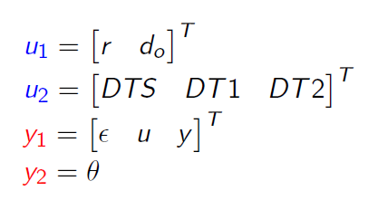
In such a configuration, the partition of the inputs and the outputs has the following signification: u1 - external inputs (disturbances, noises, references); u2 - controlled inputs;
y1 - controlled outputs (errors to be minimized, control signals to be bounded); y2 - measured outputs. In the case of the current application, this translates into:
The closed-loop system is obtained by connecting the controller to the generalized system as in Figure 3.4.1.
Figure 3.4.2 Closed loop system
The purpose of the H2/H∞ controller computing can be now expressed as: Given a generalized system T with the corresponding partitions of the inputs and the ouputs, the H2/H∞ algorithms design the controller K which measures the system output y2 and computes suitable commandu2. In the same time, the controller K must be computed in order to ensure a stable closed loop system Ty1u1 and such that it minimizes the H2 norm of the closed loop system; respectively it bounds the H∞ norm of the closed loop system, ||Ty1u1 ||∞ < γ, for a given γ > 0.
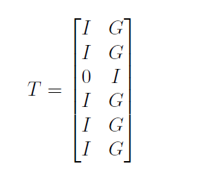
Considering the imposed performance requirements the generalized system is written in the following form:
T represents the system in the generalized form, 1 stands for the number of outputs to be measured and 3 stands for the number of inputs to be controlled. G denotes the transfer function associated with the state-space representation of the system. A discretization procedure is applied in this case too.
All the procedure described explicitly for solving the H2 control problem is applicable for the H∞ suboptimal problem too. The only difference is made by the Matlab command
which computes the controller which is now hinfsyn and used as:
4. Results and Conclusions
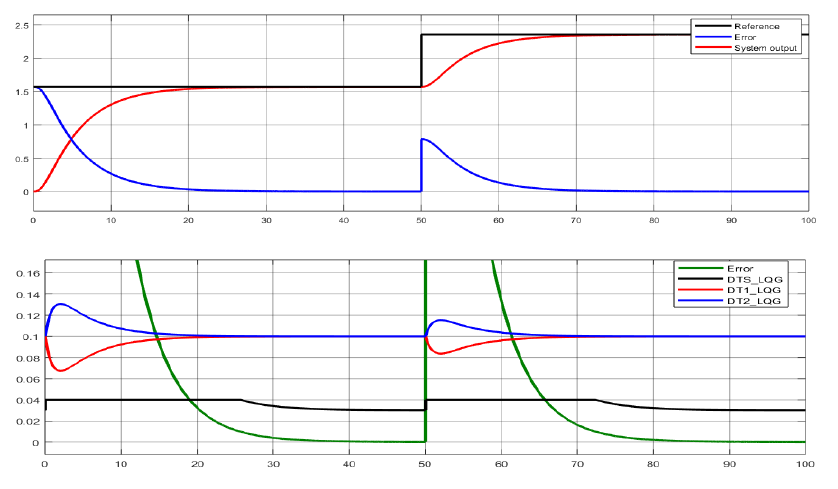
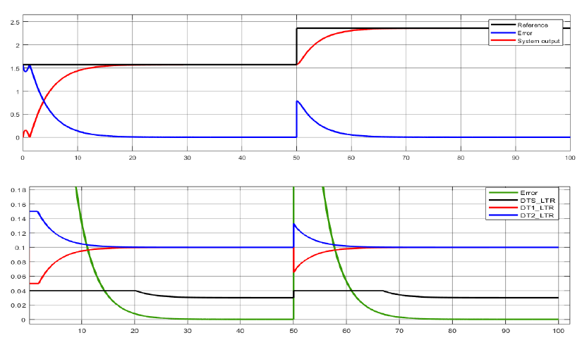
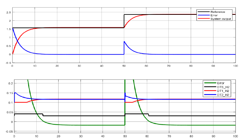
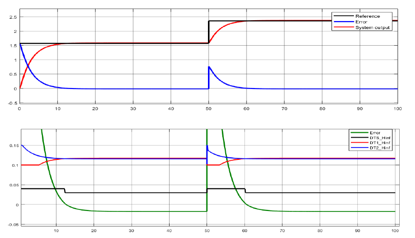
For each of the computed controllers, simulations are realized to validate their functionality on the given system. Each closed loop is analyzed for a step reference signal and the results are illustrated in the figures below:
Figure 4.1 Reference tracking and control signals computed by the LQG controller for a step reference
Figure 4.2 Reference tracking and control signals computed by the LTR controller for a step reference
Figure 4.3 Reference tracking and control signals computed by the H2 controller for a step reference
Figure 4.4 Reference tracking and control signals computed by the H∞ controller for a step reference
The signals evolution over time, as noticeable in the illustrated graphics, does not highlight significant differences between the designed control algorithms. Control signals evolution over time also reflects with accuracy the real behavior of the car. For a positive error, one of the duty cycles of the rear wheels increases, while the other one decreases. For a negative error, they change their evolution symmetrically, thus differentiating between the two types of turning, to the left, respectively to the right. In the same time, the duty cycle control signal given to the servomotor shows a variation between 0.04 for a positive error and 0.02 for a negative one, keeping its values constant at 0.03 when no error is computed.
However, H2 and H∞ algorithms represent powerful tools which do not exhibit their full-capacity advantages due to the low complexity of the system’s model. Therefore, a proportionate effort should be put into solving a real-life problem, considering its complexity and performance requirements. The LQG and LTR can also be interpreted as a particular case of the H2 control problem, as detailed in, this explaining the similarity between the time domain solutions between these two algorithms and H2. When it comes to the H∞ method, no significant advantages are enlightened by the time domain graphical evolution either. What is yet remarkable at this control option is represented by the advantages presented in the case of unstructured perturbations affecting the system’s model. As already mentioned in the paper, the nominal model approximates the real system. Therefore a behavioral uncertainty is present throughout the entire design process. Robustness related to this estimations is achieved with the H∞ control option.
However, a statistical comparison is illustrated in the following table, which contains the values of the step-response characteristics, computed for the closed loop systems. Considering that the sampling time used for the simulation is equal to 0.02s, as mentioned in the previous chapter, the results are as in the following table:
| LQG | LTR | H2 | H∞ | |
|---|---|---|---|---|
| RiseTime | 0.016s | 0.0121s | 0.0076s | 0.0068s |
| SettlingTime | 0.022s | 0.0196s | 0.015s | 0.0144s |
Table 4.1 Step-response characteristics for the closed loop system
The required performances are accomplished both with the classical and modern approaches. As concluded previously from the simulation results, no noticeable differences are in the real behavior of the four algorithms illustrated in the current chapter. The system’s model influences the car behavior slightly, compared to the classical PID perspective. Considering the neglect of some of the forces which affect the system, together with model parameters approximation, these results are as expected. Improved performances can be achieved as a future work by including the model uncertainties in a H∞ controller design procedure.
