- NXP Forums
- Product Forums
- General Purpose MicrocontrollersGeneral Purpose Microcontrollers
- i.MX Forumsi.MX Forums
- QorIQ Processing PlatformsQorIQ Processing Platforms
- Identification and SecurityIdentification and Security
- Power ManagementPower Management
- MCX Microcontrollers
- S32G
- S32K
- S32V
- MPC5xxx
- Other NXP Products
- Wireless Connectivity
- S12 / MagniV Microcontrollers
- Powertrain and Electrification Analog Drivers
- Sensors
- Vybrid Processors
- Digital Signal Controllers
- 8-bit Microcontrollers
- ColdFire/68K Microcontrollers and Processors
- PowerQUICC Processors
- OSBDM and TBDML
-
- Solution Forums
- Software Forums
- MCUXpresso Software and ToolsMCUXpresso Software and Tools
- CodeWarriorCodeWarrior
- MQX Software SolutionsMQX Software Solutions
- Model-Based Design Toolbox (MBDT)Model-Based Design Toolbox (MBDT)
- FreeMASTER
- eIQ Machine Learning Software
- Embedded Software and Tools Clinic
- S32 SDK
- S32 Design Studio
- Vigiles
- GUI Guider
- Zephyr Project
- Voice Technology
- Application Software Packs
- Secure Provisioning SDK (SPSDK)
- Processor Expert Software
-
- Topics
- Mobile Robotics - Drones and RoversMobile Robotics - Drones and Rovers
- NXP Training ContentNXP Training Content
- University ProgramsUniversity Programs
- Rapid IoT
- NXP Designs
- SafeAssure-Community
- OSS Security & Maintenance
- Using Our Community
-
-
- Home
- :
- Model-Based Design Toolbox (MBDT)
- :
- MBDT for RADAR
- :
- RADAR Systems Design and Programming Made Simple with NXP’s Model-Based Design Toolbox
RADAR Systems Design and Programming Made Simple with NXP’s Model-Based Design Toolbox
- Subscribe to RSS Feed
- Mark Topic as New
- Mark Topic as Read
- Float this Topic for Current User
- Bookmark
- Subscribe
- Mute
- Printer Friendly Page
RADAR Systems Design and Programming Made Simple with NXP’s Model-Based Design Toolbox
- Mark as New
- Bookmark
- Subscribe
- Mute
- Subscribe to RSS Feed
- Permalink
- Report Inappropriate Content
INTRODUCTION
Even though the purpose of this article is to familiarize you with SPT simulator for MATLAB, this being the first release we want to start it off by putting some things into context. In this article, we'll begin by giving you an overview of what RADAR is, where it is used and how it is different than other technologies like vision or LIDAR.
In the second part we'll be talking about a solution for RADAR developed by NXP and how it uses specialized hardware accelerators for signal processing. The final part will cover the newly released SIMULATOR for Signal Processing Toolbox (the hardware accelerator that resides on NXP’s RADAR products) and why it is easier to develop your algorithms on it, rather than on the real hardware (how it helps with visualizing data, rapidly changing parameters/steps used, saving time – thus decreasing time-to-market) – all with the help of an example, using a simulation of a radar signal to show one method you could use to find the objects in the proximity of the car, the distance to them and their relative velocity.
WHAT IS RADAR?
RADAR is a key component of ADAS (Advanced Driver Assistance Systems) that constantly senses the objects in the proximity of the car – it can determine the distance to them, their relative velocity and the angle.
RADAR improves driving efficiency and safety, being used for collision detection, warning and avoidance, blind spot monitoring, lane change assistance, rear cross-traffic alerts, vulnerable road user detection, adaptive cruise control, etc.
Figure 1 General RADAR use
Currently there are 4 major technologies which provide external and immediate information to autonomous and semi-autonomous vehicles:
- RADAR: a system that uses radio waves to determine the range, angle and velocity of objects
- Vision: a system that uses sophisticated object detection algorithms to understand what is visible from the cameras
- LIDAR (Light Detection and Ranging): technology that uses light in the form of a pulsed laser to measure ranges (distances)
- Ultrasonic: a system that uses ultrasonic sound waves to detect the distance to objects
Each one of them has advantages and disadvantages, this being the reason why we usually see them used in tandem. Let’s talk more about the ups and downs of using Radar technology:
First of all, RADAR is computationally lighter than vision and uses far less data than a LIDAR. Even though it is less angularly accurate than LIDAR, it can work regardless of the weather condition and even use reflection to see behind obstacles. This means that while LIDAR and vision struggle with bright light, night, snow, fog, dust and rain, RADAR maintains the same performances. Because of this, companies like Tesla believe it can be used not just as a supplementary sensor to the image processing system, but as a primary control sensor, maybe not even requiring confirmation from the camera:
“The radar was added to all Tesla vehicles in October 2014 as part of the Autopilot hardware suite, but was only meant to be a supplementary sensor to the primary camera and image processing system. After careful consideration, we now believe it can be used as a primary control sensor without requiring the camera to confirm visual image recognition.” (Tesla team)
RADAR COMPONENTS
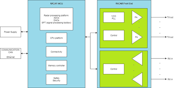
A typical RADAR module consists of a transmit solution (Tx), a voltage-controlled oscillator (VCO) and a multiple-channel receiver IC (Rx), along with a MCU. The main controller and modulation master is a single MCU with integrated high-speed analog-to-digital converters (ADCs) and appropriate signal processing capability, such as Fast Fourier Transforms (FFTs).
Figure 2 Typical Radar components
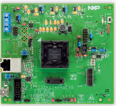
Let us look at a concrete example: NXP’s S32R274 EVB (Evaluation board):
Figure 3 S32R274
This is a 32-bit Power Architecture based Microcontroller Unit (MCU) that supports surround radar and mid-range front radar applications. It is designed to address advanced radar signal processing capabilities combined with automotive MCU capabilities for generic software tasks and car bus interfacing.
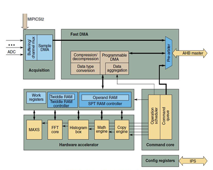
S32R274 supports radar signal processing acceleration via the Signal Processing Toolbox (SPT). This is a powerful engine containing high-performance signal processing operations (like FFT, peak search, etc.). The SPT is connected to the device by an Advanced High-Performance master bus and a peripheral bus (system bus master interface is used for fast data transfers between external memory and local RAM, while the purpose of the peripheral interface is to set configuration, get status information, basic control of SPT and trigger interrupts).
Figure 4 SPT Block Diagram
The SPT Programmable Direct Memory Access (PDMA) is one of the key elements supporting the transfer of data streams into and out of the SPT core.
Some other features of the SPT are:
- ADC sampling within programmed window
- Hardware acceleration for FFT, Histogram calculation, peak search, mathematical operations on vector data
- Compression/decompression (@data transfers)
- High-level commands for signal processing operations
- CPU interrupt notification
- Watchdog
SPT (Signal Processing Toolbox) SIMULATOR for MATLAB
To simplify the development process of radar applications, we decided to expose SPT Simulator functionality into MATLAB environment. This way, if you want to check out functionalities of SPT or even test out your algorithm by plotting step by step some intermediary data so you can fine-tune it, it will be as easy as running a regular MATLAB m-script.
Another thing worth mentioning is that this is a bit-exact simulator – so you can use native MATLAB functions to build your algorithm (resulting a Golden Model, due to the precision provided by having floating point) and use the simulator to build a Reference Model. This way you can use the toolbox for running different performance tests for your Radar application even without having to get the hardware out of the box.
Now let’s see how a Radar application looks like in our SPT Toolbox:
SPT Radar Application Example
Note: To successfully run the following example you need some Radar SDK functions. These can be found into
[..]\ {RADAR SDK INSTALL PATH}\ Tools\ SPT_bitexact_model\ src
To use them, simply download the RSDK package and add that folder to the MATLAB path.
The Radar SDK is available for download in your Software Account .
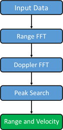
This example shows a possible way to detect the objects in front of the radar, the distance to them and their relative velocity. This method involves the following steps:
Figure 5 Radar application example – steps
Step 1: Input data
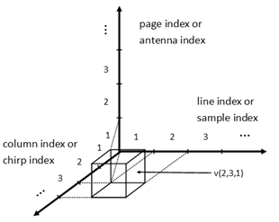
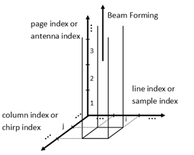
Input data is a 3-dimensional array made up of a demodulated signal. There is a page for each antenna, containing a matrix where each column contains the samples of a chirp.
NOTE: In MATLAB, we refer to the third dimension as pages. For example v(:,:,1) is the first page of v.
NOTE2: A chirp is a signal in which the frequency increases or decreases with time.
Figure 6 Input data structure
The MATLAB code for generating the input data and initializing some other variables:
% Round and saturate function
function out = round_and_saturate(in, nbits)
out = max(min(round(in * 2^(nbits-1)), 2^(nbits-1)-1), -2^(nbits-1)) / 2^(nbits-1);
End
% Number of bits used to retain the operands
NBITS = 16;
% Maximum range that can be detected
max_range = 150;
% The radar can also detect the negative velocities and its range is in
% fact [-max_velocity, max_velocity].
max_velocity = 100;
% Number of samples per chirp
M = 512;
% Number of chirps
N = 256;
% Number of antennas
P = 4;
% We take as input a 3D sine wave. This is the case when there is only one
% object in front of the radar.
% The frequency in the first dimension or the frequency of each chirp
fs = 150.5 / M;
% The frequency in the second dimension
fc = -99.5 / N;
% The frequency in the third dimension
fa = 1.5 / P;
ts = (0:M-1)';
tc = 0:N-1;
ta(1, 1, :) = 0:P-1;
ts = repmat(ts, [1, N, P]);
tc = repmat(tc, [M, 1, P]);
ta = repmat(ta, [M, N, 1]);
% Input data
input_data = sin(2*pi*(fs*ts + fc*tc + fa*ta));
% Input data as 16 bits fixed-point data
input_data_rs = round_and_saturate(input_data, NBITS);
Once we have the input data ready, we can take the next step:
Step 2: Range FFT (Fast Fourier Transform)
The FFT is an algorithm that samples a signal over a period of time and divides it into its fundamental frequency components.
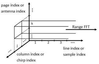
The output array of the range FFT is obtained by replacing each column of the input array with its Fourier transform. From each such Fourier transform one could deduce the ranges of all objects found in front of the radar.
Figure 7 Range FFT
Here is the MATLAB code for range FFT:
% Generate window coefficients for range FFT
% In the radar application, the signals of interest are narrowband
% sinusoids of widely differing strengths (primarily as a consequence of
% the inverse fourth power variation in radar signal strength with radar
% range) and the usage of a window function with low sidelobes is
% crucial for preventing one or more powerful signals from drowning out
% weaker reflectors.
window_rangeFFT = reshape(window('chebwin', M), [], 1);
window_rangeFFT_rs = round_and_saturate(window_rangeFFT, NBITS);
% Generate twiddle coefficients for range FFT
% The user needs only to define twiddles for one octant (- Imaginary, + Real)
% and the SPT logic determines other needed twiddles by real / imaginary
% swaps and sign inversions.
t = (1:M/8)/M;
twiddle_real = round_and_saturate(cos(-2*pi*t), NBITS);
twiddle_imag = round_and_saturate(sin(-2*pi*t), NBITS);
twiddle_rangeFFT = twiddle_real + 1i * twiddle_imag;
% Perform Range FFT
% For each line a FFT is performed. The negative frequencies are discarded.
% The frequencies with significant magnitudes indicates the presents of an
% object at a specific distance. The distance is proportional with the
% frequency.
% Non bit-exact model
exwindow_rangeFFT = repmat(window_rangeFFT, [1, N, P]);
output_rangeFFT = fft(input_data .* exwindow_rangeFFT, [], 1);
output_rangeFFT = output_rangeFFT(1:end/2, :, :) / M;
% Bit-exact model
output_rangeFFT_bitexact = rangeFFT(input_data_rs * 2^(NBITS-1), window_rangeFFT_rs * 2^(NBITS-1), twiddle_rangeFFT * 2^(NBITS-1), M, N, P);
output_rangeFFT_bitexact = output_rangeFFT_bitexact / 2^(NBITS-1);
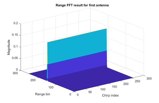
Figure 8 Range FFT Results
Step 3: Doppler FFT
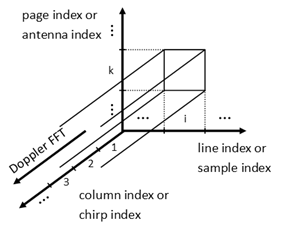
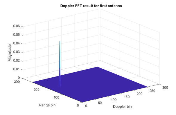
Doppler FFT has as input the output array of the range FFT. Similar with the range FFT case, the Doppler FFT output array is obtained by replacing each line of the input array with its Fourier transform. From each such Fourier transform one could deduce the velocities of all objects found in front of the radar. Moreover, from the matrix of each page one could deduce the distinct pairs of (range, velocity) of all objects found in front of the radar.
Figure 9 Doppler FFT
Here is the MATLAB code for Doppler FFT :
% Generate window coefficients for Doppler FFT
window_dopplerFFT = reshape(window('chebwin', N), [], 1);
window_dopplerFFT_rs = round_and_saturate(window_dopplerFFT, NBITS);
% Generate twiddle coefficients for Doppler FFT
t = (1:N/8)/N;
twiddle_real = round_and_saturate(cos(-2*pi*t), NBITS);
twiddle_imag = round_and_saturate(sin(-2*pi*t), NBITS);
twiddle_dopplerFFT = twiddle_real + 1i * twiddle_imag;
% Perform Doppler FFT
% For each column a FFT is performed. The frequencies with significant
% magnitudes indicates the presents of an object with a specific velocity.
% The velocity is proportional with the frequency.
% Non bit-exact model
exwindow_dopplerFFT = repmat(reshape(window_dopplerFFT, 1, []), [M/2, 1, P]);
output_dopplerFFT = fft(output_rangeFFT .* exwindow_dopplerFFT, [], 2) / N;
output_dopplerFFT = [output_dopplerFFT(:, end/2 + 1:end,:) output_dopplerFFT(:, 1:end/2, :)];
% Bit-exact model
output_dopplerFFT_bitexact = dopplerFFT(output_rangeFFT_bitexact * 2^(NBITS-1), window_dopplerFFT_rs * 2^(NBITS-1), twiddle_dopplerFFT * 2^(NBITS-1), M, N, P);
output_dopplerFFT_bitexact = output_dopplerFFT_bitexact / 2^(NBITS-1);
Figure 10 Doppler FFT Results
Step 4: Peak search
Peak search detects the magnitude peaks of the matrix obtained from beam forming. The beam forming cancels the time delay between the signals of any group of two adjacent antennas and adds the resulted signals. This is accomplished by performing a FFT on all vectors obtained in the following manner: for a pair [line index; column index] get the samples from all pages.
Figure 11 Peak search
Here is the MATLAB code for peak search :
% Generate twiddle coefficients for peak search
t = (1:16/8)/16;
twiddle_real = round_and_saturate(cos(-2*pi*t), NBITS);
twiddle_imag = round_and_saturate(sin(-2*pi*t), NBITS);
twiddle_peakSearch = twiddle_real + 1i * twiddle_imag;
% Perform Peak Search
% Non bit-exact model
fftOut = fft(output_dopplerFFT, 16, 3);
fftOut = abs(fftOut / 16) .^ 2;
fftMag = squeeze(max(fftOut, [], 3));
% Compute a histogram for each range
% B - number of bins for histogram
B = 46;
rangeHistogram = zeros(M/2, B);
edges = [0 2.^(-B+1: 0)];
for m = 1:M/2
[tmpHist, ~] = histcounts(fftMag(m, :), edges);
rangeHistogram(m, :) = tmpHist;
end
% Determine a threshold for each range
threshold = ones(1, M/2);
for m = 1:M/2
tmpHist = rangeHistogram(m, :);
[~, ind] = max(tmpHist);
while(tmpHist(ind) ~= 0)
ind = ind + 1;
end
threshold(m) = 2^(ind - B);
end
peakTag = zeros(M/2, N);
% Tag peaks over each range gate
for m = 1:M/2
cGate = fftMag(m, :);
peakTag(m, 1) = (cGate(end) < cGate(1)) && (cGate(1) >= cGate(2));
for n = 2:N-1
peakTag(m, n) = (cGate(n-1) < cGate(n)) && (cGate(n) >= cGate(n+1));
end
peakTag(m, n+1) = (cGate(n) < cGate(end)) && (cGate(end) >= cGate(1));
end
% Tag peaks over each Doppler gate
for n = 1:N
cGate = fftMag(:, n);
peakTag(1, n) = peakTag(1, n) && (cGate(1)>=cGate(2));
for m = 2:M/2-1
peakTag(m, n) = peakTag(m, n) && (cGate(m-1) <cGate(m) ) && (cGate(m)>=cGate(m+1));
end
peakTag(m+1, n) = peakTag(m+1, n) && (cGate(m)<cGate(m+1));
end
% Detect peaks above threshold
thresholdTag = zeros(size(peakTag));
for m = 1:M/2
thresholdTag(m, :) = fftMag(m, :) > threshold(m);
end
output_peakSearch = peakTag .* thresholdTag;
% Bit-exact model
[output_peakSearch_bitexact, OutScratch] = peakSearch3D(output_dopplerFFT_bitexact * 2^(NBITS-1), twiddle_peakSearch * 2^(NBITS-1), threshold * 2^(B-1), M/2, N, P);
Step5: Range and Velocity
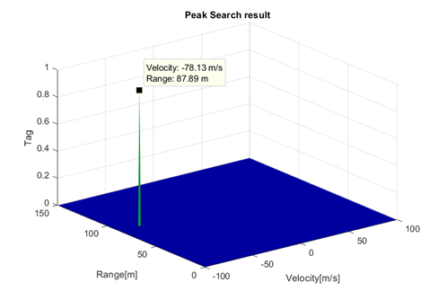
The result matrix contains all detectable ranges(line-indexed), and all detectable velocities (column- indexed). The matrix contains only 1s and 0s. Each element that has the value 1 corresponds to at least one detected object and its velocity and range are given by its coordinates.
So, if we use this plot we will get the following image:
figure; mesh(max_velocity * (-N:2:N-2)/N, max_range * (0:2:M-2)/M, output_peakSearch_bitexact);
title('Peak Search result');
xlabel('Velocity'); ylabel('Range'); zlabel('Tag');
Figure 12 Peak search result
This shows an object coming towards the radar with 78.13 m/s velocity, being at that moment at 87.89m away.
So, this example shows a simple method for simulating the implementation of a Radar application (starting with a demodulated input, performing range and Doppler FFT and a peak search to get object’s velocity and range, relative to the Radar).
Ending note
Why use this toolbox? Because you can easily change any variable, at any step and instantly see how it impacts your algorithm, all of this without having to worry about nothing (hardware-related).
In this current context, where time-to-market is a big deal, the opportunity of a speed-up for the development of various applications should be worth taking.
| How to Detect Objects With RADAR Using NXP's Model-Based Design Toolbox | ||
|---|---|---|
NOTE: Chinese viewers can watch the video on YOUKU using this link 注意:中国观众可以使用此链接观看YOUKU上的视频 | ||
UPDATE May 11th, 2018: for latest Radar SDK version 0.9.0 the new MATLAB script attached bellow as demo_4antennas_video_RSDKv090.m shall be used.
UPDATE October 11th, 2018: for latest Radar SDK version 1.1.1 the new MATLAB script attached bellow as demo_4antennas_video_RSDKv1_1_1.m shall be used.

