- NXP Forums
- Product Forums
- General Purpose MicrocontrollersGeneral Purpose Microcontrollers
- i.MX Forumsi.MX Forums
- QorIQ Processing PlatformsQorIQ Processing Platforms
- Identification and SecurityIdentification and Security
- Power ManagementPower Management
- MCX Microcontrollers
- S32G
- S32K
- S32V
- MPC5xxx
- Other NXP Products
- Wireless Connectivity
- S12 / MagniV Microcontrollers
- Powertrain and Electrification Analog Drivers
- Sensors
- Vybrid Processors
- Digital Signal Controllers
- 8-bit Microcontrollers
- ColdFire/68K Microcontrollers and Processors
- PowerQUICC Processors
- OSBDM and TBDML
-
- Solution Forums
- Software Forums
- MCUXpresso Software and ToolsMCUXpresso Software and Tools
- CodeWarriorCodeWarrior
- MQX Software SolutionsMQX Software Solutions
- Model-Based Design Toolbox (MBDT)Model-Based Design Toolbox (MBDT)
- FreeMASTER
- eIQ Machine Learning Software
- Embedded Software and Tools Clinic
- S32 SDK
- S32 Design Studio
- Vigiles
- GUI Guider
- Zephyr Project
- Voice Technology
- Application Software Packs
- Secure Provisioning SDK (SPSDK)
- Processor Expert Software
-
- Topics
- Mobile Robotics - Drones and RoversMobile Robotics - Drones and Rovers
- NXP Training ContentNXP Training Content
- University ProgramsUniversity Programs
- Rapid IoT
- NXP Designs
- SafeAssure-Community
- OSS Security & Maintenance
- Using Our Community
-
-
- Home
- :
- Model-Based Design Toolbox (MBDT)
- :
- MBDT for RADAR
- :
- Accelerate the Discrete Fourier Transform with NXP SPT
Accelerate the Discrete Fourier Transform with NXP SPT
- Subscribe to RSS Feed
- Mark Topic as New
- Mark Topic as Read
- Float this Topic for Current User
- Bookmark
- Subscribe
- Mute
- Printer Friendly Page
Accelerate the Discrete Fourier Transform with NXP SPT
- Mark as New
- Bookmark
- Subscribe
- Mute
- Subscribe to RSS Feed
- Permalink
- Report Inappropriate Content
 |
Theoretical background
A Discrete Fourier Transform (DFT) converts a signal from time domain (left) into frequency domain (right). Every signal is made of one or multiple frequencies. If you consider a sound wave, then any sample of that sound wave has a set of frequencies with corresponding amplitudes that describe the overall sound wave.
Fourier demonstrated that you can take a set of sinusoids of different amplitudes and frequencies and by adding them together you can build up any signal - including a square one if needed. A plot of frequency versus amplitude on an x-y graph of these sinusoids represents a frequency spectrum, or frequency domain plot.
INTRODUCTION
In this article we are going to discuss about how to compute the DFT of real signals using the FFT (Fast Fourier Transform) algorithm. The FFT algorithm is implemented using the instructions RDX2 and RDX4.
To explain why we need to compute the DFT in RADAR, let us take the simplest scenario. Suppose that we have only one object in front of the RADAR, then the demodulated signal from a chirp is a sinusoid. The frequency of the sinusoid is proportional to the range between the RADAR and the object. To find the frequency of the sinusoid we compute its DFT. For positive frequencies the DFT will have only one peak. The peak is at the frequency of the sinusoid.
SPT INPUT DATA
Data received by the SPT is made of demodulated signal and can be organized as a 3-dimensional array in the following way: there is a page for each antenna, and each page contains a matrix where each column contains the samples of a chirp.
In MATLAB we refer to the third dimension as pages. For example v(:,:,1) is the first page of v.
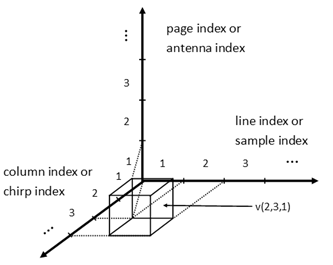 |
| Fig. 1: SPT input data representation |
% Number of bits used to retain the operands
NBITS = 16;
% Number of samples per chirp
M = 512;
% Number of chirps
N = 256;
% Number of antennas
P = 4;
% We take a input a 3D sine wave. This is the case when there is only one
% object in front of the radar.
% The frequency in the first dimension or the frequency of each chirp
fs = 50.5 / M;
% The frequency in the second dimension or the Doppler frequency
fc = -99.5 / N;
% The frequency in the third dimension
fa = 1.5 / P;
ts = (0:M-1)';
tc = 0:N-1;
ta(1, 1, : )= 0:P-1;
ts = repmat(ts, [1, N, P]);
tc = repmat(tc, [M, 1, P]);
ta = repmat(ta, [M, N, 1]);
% Input data
input_data = sin(2*pi*(fs*ts + fc*tc + fa*ta));
% Input data as 16 bits fixed-point data
input_data_rs = round_and_saturate(input_data, NBITS) * 2^(NBITS-1);
RANGE FFT
The output array of the range FFT is obtained by replacing each column of the input array with its DFT. As described in the introduction, from each such DFT one can find the ranges of all objects found in front of the RADAR.
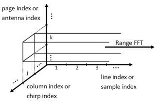 |
| Fig. 2: Range FFT input data processing |
DATA PROCESSING FLOWCHART
Because the demodulated signal is real, the range FFT can be sped-up by computing the DFTs of two real signals at once. This is done by computing the DFT of the complex signal which has on the real part the first signal and on the imaginary part the second one, and then split the resulted DFT.
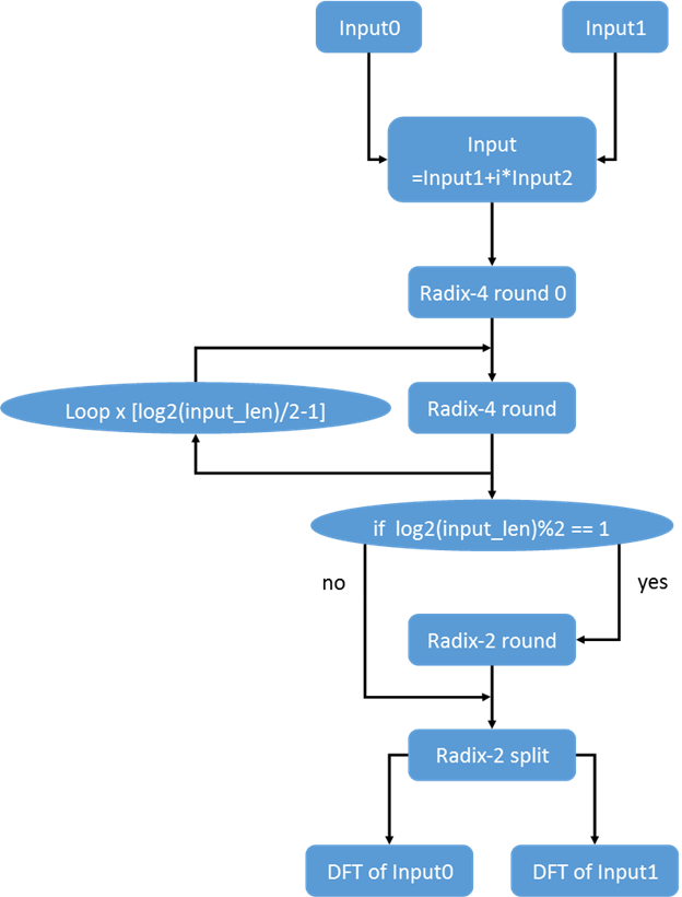 |
| Fig. 3: FFT algorithm data processing flowchart |
FFT INPUT DATA
The FFT input data is made of the second chirp of the first two antennas.
% First real input is the second chirp from first antenna
input0 = input_data_rs(:, 2, 1);
% Second real input is the second chirp from second antenna
input1 = input_data_rs(:, 2, 2);
input = input0 + 1i * input1;
Below are the two real inputs. It can be observed that the two inputs are sinusoids with the same frequency, but different phase.
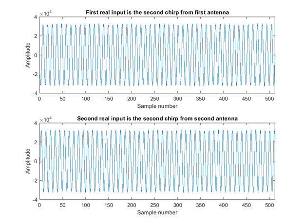 |
| Fig. 4: FFT input data |
FFT PROCESSING
One radix-4 is done using the instruction RDX4, and one radix-2 round is done using the instruction RDX2. The first round of the FFT is a radix-4 round. In this round, because there is no need of twiddle factors, the instruction RDX4 lets you apply a window function on the input sequence. After we apply the remaining radix-4 rounds, if needed, we apply one radix-2 round. The last step is to find the DFTs of the real signals. This is done using the instruction RDX2.
% Deduce the number of radix-4 rounds and if there is a radix-2 round
input_length = numel(input);
log2_input_length = log2(input_length);
num_rdx4_rounds = floor(log2_input_length / 2);
num_rdx2_rounds = mod(log2_input_length, 2);
num_rounds = num_rdx4_rounds + num_rdx2_rounds;
% Twiddle factors
t = (1:input_length/8)/input_length;
M_Tw_real = round_and_saturate(cos(-2*pi*t), NBITS) * 2^(NBITS-1);
M_Tw_imag = round_and_saturate(sin(-2*pi*t), NBITS) * 2^(NBITS-1);
M_Tw = M_Tw_real + 1i * M_Tw_imag;
% Results
M_Out = zeros(num_rounds + 1, input_length);
% Windowing operation - Indicates whether or not is the window multiplication
% enabled
win_type = 'WIN_DISABLED';
% Win coefficient type - Indicates the type of window coefficients
win_coeff_type = 'MULTIPLE_COEFF'; % do not care
% Quadrature Extension
quad_ext = 'QUAD_EXT';
% Repeat - Decides whether combined fft operation is enabled or not
repeat = 'NO_COMBINED_FFT';
% Pre-scaling left shift value
shft_val = 0;
% FFT Round
fft_rnd = 0;
% Window function
M_Wc = 0;
% Operands
M_Op = input;
% Result
M_Out(1, : )= rdx4_mex(complex(M_Wc), complex(M_Op), win_type, win_coeff_type, fft_rnd, quad_ext, repeat, shft_val);
for i = 1:num_rdx4_rounds-1
% FFT Round
fft_rnd = i;
% Operands values
M_Op = M_Out(i, :);
% Result
M_Out(i+1, : )= rdx4_mex(M_Tw, M_Op, win_type, win_coeff_type, fft_rnd, quad_ext, repeat, shft_val);
end
% rdx2 round
if num_rdx2_rounds ~= 0
% FFT Round
fft_rnd = num_rounds - 1;
% Real FFT
real_fft = 'NO_OPERANDS_SPLIT';
% Quadrature Extension
quad_ext = 'QUAD_EXT';
% Repeat
repeat = 'NO_COMBINED_FFT';
% Pre-scaling left shift value
shft_val = 0;
% Operands values
M_Op = M_Out(num_rounds - 1, :);
% Result
M_Out(num_rounds, : )= rdx2_mex(M_Tw, M_Op, fft_rnd, real_fft, quad_ext, repeat, shft_val);
end
% DFT split
% FFT Round
fft_rnd = num_rounds - 1;
% Real FFT
real_fft = 'OPERANDS_SPLIT';
% Quadrature Extension
quad_ext = 'QUAD_EXT';
% Repeat
repeat = 'NO_COMBINED_FFT';
% Pre-scaling left shift value
shft_val = 0;
% Operands values
M_Op = M_Out(num_rounds, :);
% Result
M_Out(end, : )= rdx2_mex(M_Tw, M_Op, fft_rnd, real_fft, quad_ext, repeat, shft_val);
RESULTS
We verify the results using the FFT MATLAB function. In the image below the first column displays the magnitude of the two DFTs, and the second column displays their phases.
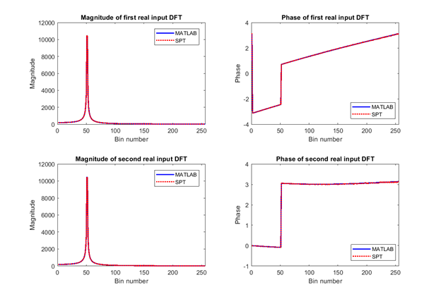 |
| Fig. 5: Magnitude and Phase DFT of the real input signals |
The script used in this example is attached below.
We hope you find this information useful. Feel free to LIKE this article and comment below.
- Mark as New
- Bookmark
- Subscribe
- Mute
- Subscribe to RSS Feed
- Permalink
- Report Inappropriate Content
In Doppler FFT , it need to apply on result of Range FFT .
For this how to consider input signal combination to FFT.