- NXP Forums
- Product Forums
- General Purpose MicrocontrollersGeneral Purpose Microcontrollers
- i.MX Forumsi.MX Forums
- QorIQ Processing PlatformsQorIQ Processing Platforms
- Identification and SecurityIdentification and Security
- Power ManagementPower Management
- MCX Microcontrollers
- S32G
- S32K
- S32V
- MPC5xxx
- Other NXP Products
- Wireless Connectivity
- S12 / MagniV Microcontrollers
- Powertrain and Electrification Analog Drivers
- Sensors
- Vybrid Processors
- Digital Signal Controllers
- 8-bit Microcontrollers
- ColdFire/68K Microcontrollers and Processors
- PowerQUICC Processors
- OSBDM and TBDML
-
- Solution Forums
- Software Forums
- MCUXpresso Software and ToolsMCUXpresso Software and Tools
- CodeWarriorCodeWarrior
- MQX Software SolutionsMQX Software Solutions
- Model-Based Design Toolbox (MBDT)Model-Based Design Toolbox (MBDT)
- FreeMASTER
- eIQ Machine Learning Software
- Embedded Software and Tools Clinic
- S32 SDK
- S32 Design Studio
- Vigiles
- GUI Guider
- Zephyr Project
- Voice Technology
- Application Software Packs
- Secure Provisioning SDK (SPSDK)
- Processor Expert Software
-
- Topics
- Mobile Robotics - Drones and RoversMobile Robotics - Drones and Rovers
- NXP Training ContentNXP Training Content
- University ProgramsUniversity Programs
- Rapid IoT
- NXP Designs
- SafeAssure-Community
- OSS Security & Maintenance
- Using Our Community
-
-
- Home
- :
- Model-Based Design Toolbox (MBDT)
- :
- NXP Model-Based Design Tools for VISION Knowledge Base
- :
- AI and Machine Learning Course #2: Introduction to Deep Learning
AI and Machine Learning Course #2: Introduction to Deep Learning
- Subscribe to RSS Feed
- Mark as New
- Mark as Read
- Bookmark
- Subscribe
- Printer Friendly Page
- Report Inappropriate Content
AI and Machine Learning Course #2: Introduction to Deep Learning
AI and Machine Learning Course #2: Introduction to Deep Learning
1. INTRODUCTION
In this article we are going to discuss about the way the Convolutional Neural Networks are designed and maintained in the NXP Vision Toolbox and in MATLAB and offer a brief introduction of the concepts used in modern-day Machine Learning and Deep Neural Networks. This course will cover the following topics:
- CNN Architecure: concept, definition and implementation
- Perceptron: short intro and the problems it solves
- MultiLayered perceptrons
- CNN training: various CNN pre-trained architectures
Deep learning (also known as deep structured learning or hierarchical learning) is part of a broader family of machine learning methods based on the layers used in artificial neural networks. Learning can be supervised, semi-supervised or unsupervised. Deep learning is primarily a study of multi-layered neural networks, spanning over a great range of model architectures such as deep neural networks, deep belief networks, recurrent neural networks and convolutional neural networks.
It is not our intention to provide a full coverage of the deep learning topic in this topic - that would be unrealistic. If you are new to this topic then we advice you to start with:
- Short introduction - https://www.mathworks.com/discovery/deep-learning.html
- Matlab Deep Learning training - https://www.mathworks.com/learn/tutorials/deep-learning-onramp.html
2. CNN Architecture
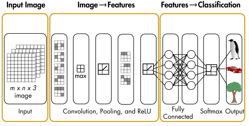
A convolutional neural network (CNN or ConvNet) is one of the most popular algorithms for deep learning, a type of machine learning in which a model learns to perform classification tasks directly from images, video, text, or sound. CNNs are particularly useful for finding patterns in images to recognize objects, faces, and scenes. Such algorithms learn directly from image data, using patterns to classify images and eliminating the need for manual feature extraction.
CNNs provide an optimal architecture for image recognition and pattern detection. Combined with advances in parallel computing, CNNs are a key technology underlying new developments in automated driving and facial recognition.
2.1 Feature Detection
A convolutional neural network can have tens or hundreds of layers that each learn to detect different features of an image. Filters are applied to each training image at different resolutions, and the output of each convolved image is used as the input to the next layer. The filters can start as very simple features, such as brightness and edges, and increase in complexity to features that uniquely define the object.
Like other neural networks, a CNN is composed of an input layer, an output layer, and many hidden layers in between. These layers perform operations that alter the data with the intent of learning features specific to the data.
Three of the most common CNN layers are:
- Convolution: puts the input images through a set of convolutional filters, each of which activates certain features from the images. The Convolution layer uses a filter matrix over the array of image pixels and performs convolution operation to obtain a convolved feature map.
- Rectified linear unit (ReLU): allows for faster and more effective training by mapping negative values to zero and maintaining positive values. This is sometimes referred to as activation, because only the activated features are carried forward into the next layer.
- Pooling simplifies the output by performing nonlinear down sampling, reducing the number of parameters that the network needs to learn
These operations are repeated over tens or hundreds of layers, with each layer learning to identify different features.
After learning features in many layers, the architecture of a CNN shifts to classification. The next-to-last layer is a fully connected layer that outputs a vector of K dimensions where K is the number of classes that the network will be able to predict. This vector contains the probabilities for each class of any image being classified.
The final layer of the CNN architecture uses a classification layer such as softmax to provide the classification output. The softmax activation function is often placed at the output layer of a neural network. It’s commonly used in multi-class learning problems where a set of features can be related to one-of-K classes. For example, in the CIFAR-10 image classification problem, given a set of pixels as input, we need to classify if a particular sample belongs to one-of-ten available classes: i.e., cat, dog, airplane, etc. Its equation is simple, we just have to compute for the normalized exponential function of all the units in the layer. Intuitively, what the softmax does is that it squashes a vector of size K between 0 and 1. Furthermore, because it is a normalization of the exponential, the sum of this whole vector equates to 1. We can then interpret the output of the softmax as the probabilities that a certain set of features belongs to a certain class.
The classification part is done using a Multi Layered Neural Network. A Multi Layered Neural Network consists of a number of layers made up out of Single Layer Perceptrons, which we will cover in the next paragraph.
2.2 Single Layer Perceptron
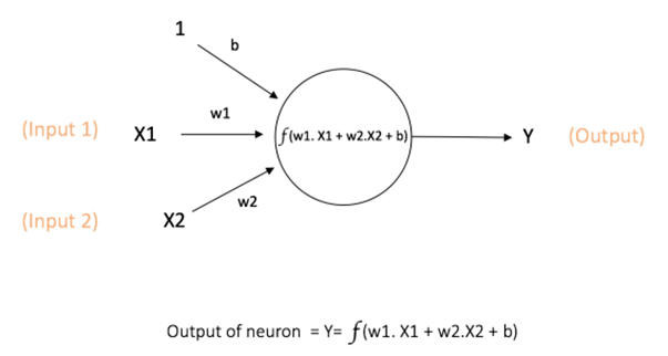
CNNs, like neural networks, are made up of neurons with learnable weights and biases. Each neuron receives several inputs, takes a weighted sum over them, passes it through an activation function and responds with an output. The basic structures of neural networks are perceptrons. The perceptron is depicted in the below figure:
The perceptron consists of weights (including a special weight called bias) , summation processor and an activation function. In same cases there is an extra input node called a bias. All the inputs are individually weighted, added together and passed into the activation function.
Every activation function (or non-linearity) takes a single number and performs a certain fixed mathematical operation on it. There are several activation functions that are encountered in practice:
- Sigmoid: takes a real-valued input and squashes it to range between 0 and 1
σ(x) = 1 / (1 + exp(−x))
- tanh: takes a real-valued input and squashes it to the range [-1, 1]
tanh(x) = 2σ(2x) − 1
- ReLU: ReLU stands for Rectified Linear Unit. It takes a real-valued input and thresholds it at zero (replaces negative values with zero)
f(x) = max(0, x)
The main function of Bias is to provide every node with a trainable constant value (in addition to the normal inputs that the node receives).
In a nutshell, a perceptron is a very simple learning machine. It can take in a few inputs, each of which has a weight to signify how important it is, and generate an output decision of “0” or “1”. More specifically it is a linear classification algorithm, because it uses a line to determine an input’s class. However, when combined with many other perceptrons, it forms an artificial neural network.
2.3 Multi Layer Perceptron
A Multi Layer Perceptron (MLP) contains one or more hidden layers (apart from one input and one output layer). While a single layer perceptron can only learn linear functions, a multi layer perceptron can also learn non – linear functions.
All connections have weights associated with them, each layer having its own bias. The process by which a Multi Layer Perceptron learns is called the backpropagation algorithm. Initially all the edge weights are randomly assigned. For every input in the training dataset, the Neural Network is activated and its output is observed. This output is compared with the desired output that we already know, and the error is “propagated” back to the previous layer. This error is noted and the weights are “adjusted” accordingly. This process is repeated until the output error is below a predetermined threshold. The process of "adjusting" the weights makes use of the Gradient Descent algorithm for minimizing the error function, which we will not go into details about.
3. CNN implementation with MATLAB and NXP Vision Toolbox
MATLAB provides an convenient & easy way to train Neural Networks from scratch using its Deep Learning Toolbox. However, this task may be daunting and may require a lot of computational resources and time. To train a deep network from scratch, you must gather a very large labeled data set and design a network architecture that will learn the features and model. This is good for new applications, or applications that will have a large number of output categories. This is a less common approach because with the large amount of data and rate of learning, these networks typically take days or weeks to train.
MATLAB also provides a series of ready-to-use pre-trained CNNs which can be customized and adapted through Transfer Learning, a topic we will cover in a chapter below. There are a few standard CNNs that one can use to classify a bunch of standard objects (such as a cat, a dog, a screwdriver, an apple and so on..). The NXP Vision Toolbox focuses on three of these pre-trained models for exemplification, but it also provides support for using others and for tailoring the above-mentioned ones.
The NXP Vision Toolbox provides a way to create Convolutional Networks using pre-trained models from MATLAB, allowing smooth and simple usage in simulation algorithms as well as straight-forward deployment on the NXP S32V234 boards. There is also the possibility of securely running the CNNs in MATLAB to classify images taken directly from the MIPI-CSI attached camera on the board needing minimal configuration steps. One should only know the IP Address of the board and assign a port for the connection to-and-from the PC. There are 3 easy ways to use the NXP Vision Toolbox for image classification using CNNS:
- Run the algorithms in simulation mode in MATLAB using the PC’s webcam
- Run the algorithms in simulation mode in MATLAB using the camera attached to the S32V234 board
- Run the algorithms on the hardware
We will get into the specifics of each of these interaction modes in a further document. In the next paragraphs we will provide a short description of the models that are available in the toolbox as examples:
3.1 GoogLeNet - Pretrained CNN
Google’s GoogLeNet project was one of the winning teams in the 2014 ImageNet large-scale visual recognition challenge (ILSVRC), an annual competition to measure improvements in machine visual technology. GoogLeNet is a pretrained convolutional neural network that is 22 layers deep. GoogLeNet has been trained on over a million images and can classify images into 1000 object categories (such as keyboard, coffee mug, pencil, and many animals). The network has learned rich feature representations for a wide range of images. The network takes an image as input, and then outputs a label for the object in the image together with the probabilities for each of the object categories.
The input size for the image is 224x224x3, but one can provide any image since the toolbox will convert it to the appropriate size.
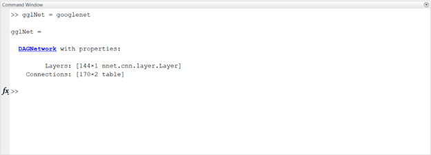
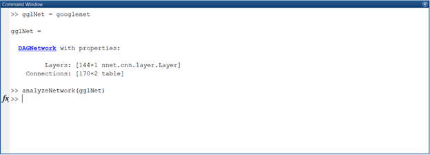
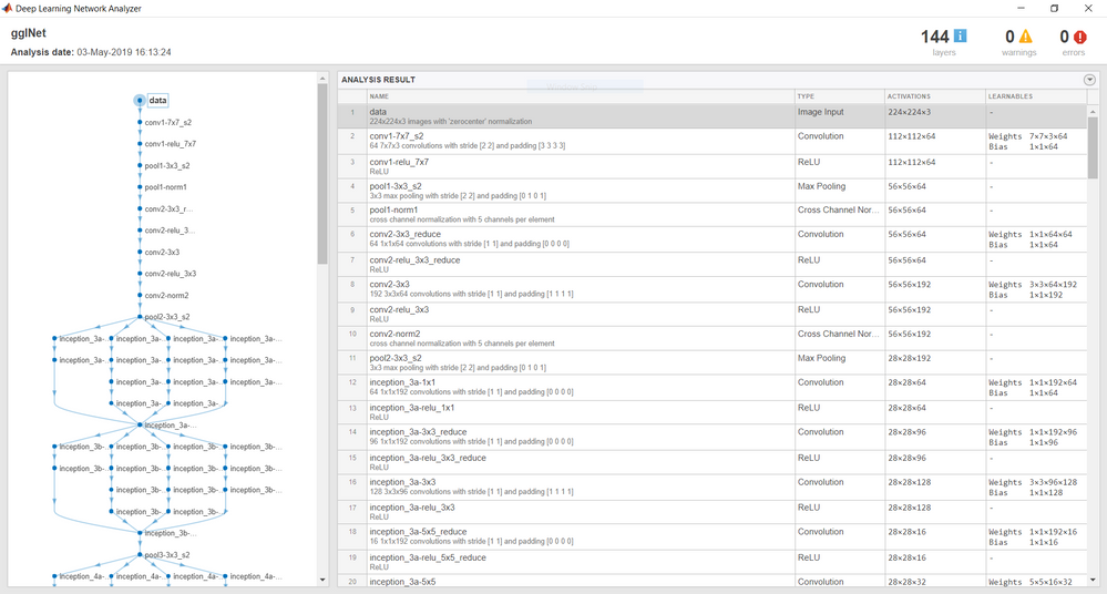
Using just the command in the above Command Window, we were able to get a hold of the GoogLeNet pretrained model in MATLAB. One can inspect the network layers in detailes by calling the analyzeNetwork function:
As you can see the network is made up of a bunch of layers connected as a DAGNetwork (Directed Acyclic Graph Network).
DAGNetwork properties:
Layers - The layers of a network
Connections - The connections between the layers
DAGNetwork methods:
predict - Run the network on input data
classify - Classify data with a network
activations - Compute specific network layer activations.
plot - Plot a diagram of the network
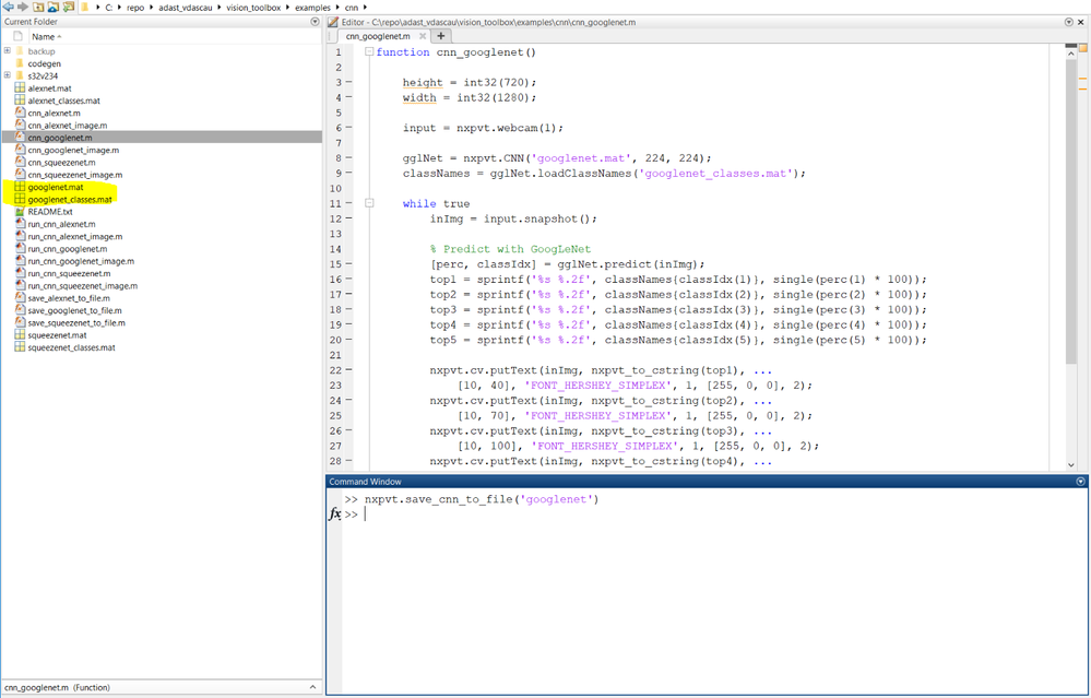
The layers are pretty much standard, except that there are some Inception layers specific to GoogLeNet. Inception layers of GoogLeNet consist of six convolution layers with different kernel sizes and one pooling layer. To create a GoogLeNet convolutional neural network object with the NXP Vision Toolbox one should get a hold of the .mat saved from the GoogLeNet object in Matlab as well as the classes within it. This can be done using the nxpvt.save_cnn_to_file(cnnObj) wrapper provided in the toolbox:
As you can see, the googlenet.mat and googlenet_classes.mat files are created which can then be used to create the nxpvt.CNN wrapper object. The creating, the simulation and the deployment of these objects and algorithms will be discussed in detail in a future document.
3.2 AlexNet - Pretrained CNN
In 2012, AlexNet significantly outperformed all the prior competitors and won the challenge by reducing the top-5 error from 26% to 15.3%. The second place top-5 error rate, which was not a CNN variation, was around 26.2%.
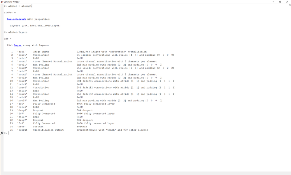
The image input size for this network in MATLAB is 227x227x3. Creating a MATLAB provided alexnet SeriesNetwork object is done with the following command:
To take a peek at the network layers use the analyzeNetwork command as above. This will display the layers with their corresponding weights and biases:
Unlike GoogLeNet, the AlexNet object is of type SeriesNetwork. A series network is one where the layers are arranged one after the other. There is a single input and a single output.
SeriesNetwork properties:
Layers - The layers of the network.
SeriesNetwork methods:
predict - Run the network on input data.
classify - Classify data with a network.
activations - Compute specific network layer activations.
predictAndUpdateState - Predict on data and update network state.
classifyAndUpdateState - Classify data and update network state.
resetState - Reset network state.
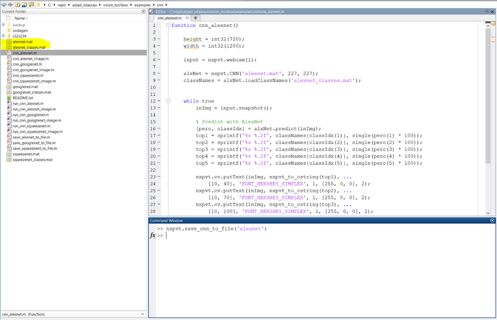
The CNN object is again created with the help of the generated .mat files:
3.3. SqueezeNet - Pretrained CNN
SqueezeNet is the name of a deep neural network that was released in 2016. SqueezeNet was developed by researchers at DeepScale, University of California, Berkeley, and Stanford University. In designing SqueezeNet, the authors' goal was to create a smaller neural network with fewer parameters that can more easily fit into computer memory and can more easily be transmitted over a computer network. SqueezeNet achieves the same accuracy as AlexNet but has 50x less weights. To achieve that SqueezeNet has following key ideas:
- Replace 3×3 filters with 1×1 filters: 1×1 have 9 times fewer parameters.
- Decrease the number of input channels to 3×3 filters: The number of parameters of a convolutional layer depends on the filter size, the number of channels, and the number of filters.
- Downsample late in the network so that convolution layers have large activation maps: This might sound counter intuitive. But since the model should be small, we need to make sure that we get the best possible accuracy out of it. The later we down sample the data (e.g. by using strides >1) the more information are retained for the layers in between, which increases the accuracy
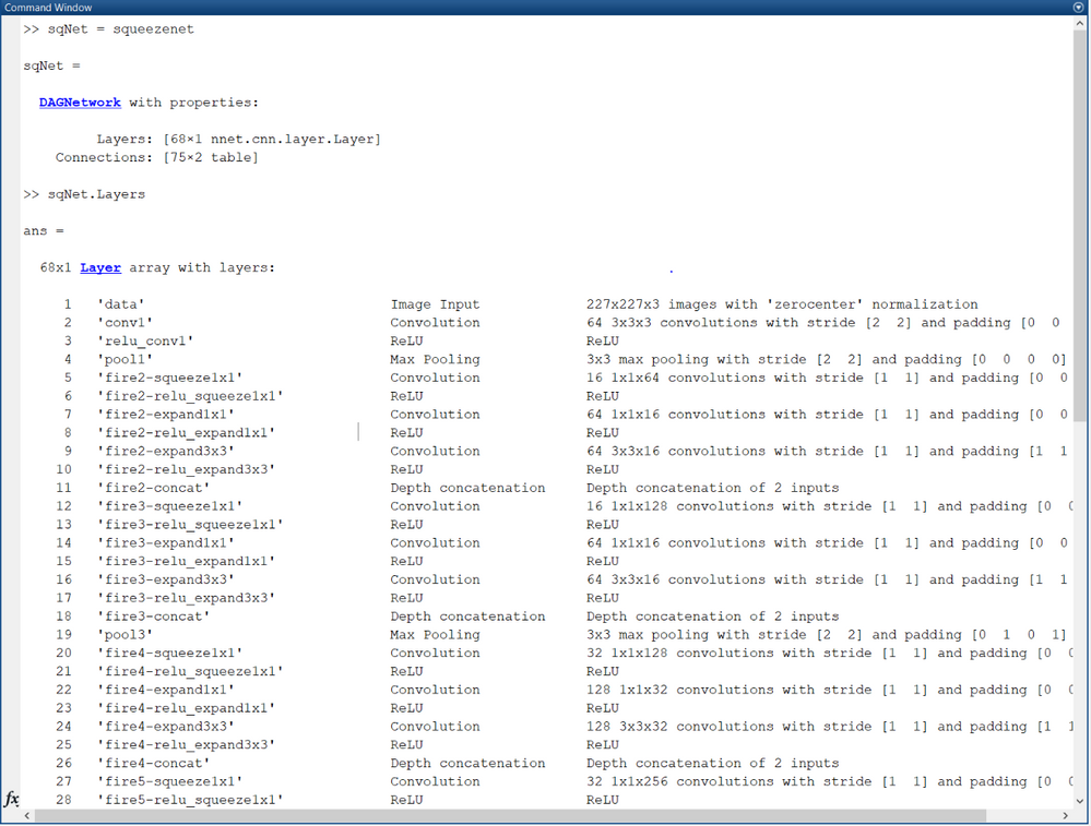
The building brick of SqueezeNet is called a fire module, which contains two layers: a squeeze layer and an expand layer. A SqueezeNet stacks a bunch of fire modules and a few pooling layers. The squeeze layer and expand layer keep the same feature map size, while the former reduces the depth to a smaller number and the latter increases it. The MATLAB implementation is a DAGNetwork, just as GoogLeNet.
Using analyzeNetwork on a squeezenet object will describe its contents:
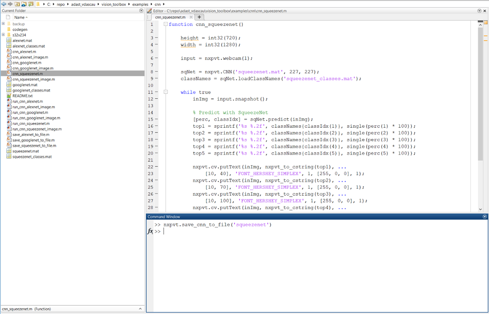
The NXP Vision Toolbox CNN object over squeezenet is created using the .mat filse generated with the nxpvt.save_cnn_to_file command.
This was a general introduction that highlights the models used by the NXP Vision Toolbox for Machine Learning on the NXP boards. To find out more about how to use the CNN examples provided in the NXP Vision Toolbox and more, please, stay tuned for our next presentations.
4. CNN Comparison & Conclusions
Pretrained networks have different characteristics that matter when choosing a network to apply to your problem. The most important characteristics are network accuracy, speed, and size.
Choosing a network is generally a tradeoff between these characteristics. A network is Pareto efficient if there is no other network that is better on all the metrics being compared, in this case accuracy and prediction time. The set of all Pareto efficient networks is called the Pareto frontier. The Pareto frontier contains all the networks that are not worse than another network on both metrics. The plot connects the networks that are on the Pareto frontier in the plane of accuracy and prediction time. All networks except AlexNet, VGG-16, VGG-19, Xception, NASNet-Mobile, ShuffleNet, and DenseNet-201 are on the Pareto frontier.

Since in this training we are going to deploy the CNN on an embedded system where we need to consider the limitations in terms of memory footprint and processing power, we've selected the first 3 CNN with the smallest size/prediction time requirements: AlexNet, SqeezeNet and GoogLeNet
For a more detailed comparison please visit: https://www.mathworks.com/help/deeplearning/ug/pretrained-convolutional-neural-networks.html
